Our goal is to simulate a mechanical system according to its Hamiltonian H ⁣(q,p,t)\mathcal H\!\left(\mathbf q,\mathbf p,t\right).

To utilize the canonical equations dqdt=Hp,dpdt=Hp,\frac{\mathrm d\mathbf q}{\mathrm dt}= \frac{\partial\mathcal H}{\partial\mathbf p},\quad \frac{\mathrm d\mathbf p}{\mathrm dt}= -\frac{\partial\mathcal H}{\partial\mathbf p}, (1)(1) we need to calculate the partial derivatives of H\mathcal H. Here is a simple code to calculate partial derivatives.

1
2
3
4
5
6
7
def div x0, dx, f
	f0 = f.(x0)
	n = x0.size
	Array.new n do |i|
		(f.(x0 + Vector.basis(n, i) * dx) - f0) / dx
	end
end

(RGSS do not have matrix.rb, you can copy one from the attached file below.) Here x0 is a Vector, f is a call-able object as a function of vectors, dx is a small scalar which we are going to take 1e-6.

Let x = Vector[*q, *p], and then Formula 1 has the form dxdt=f ⁣(x).\frac{\mathrm d\mathbf x}{\mathrm dt}=f\!\left(\mathbf x\right). To solve this equation numerically, we need to use a famous method called the (explicit) Runge–Kutta method.

1
2
3
4
5
6
7
8
def runge_kutta initial, max_t, dt, (*pyramid, coefs), func
	(0..max_t).step(dt).reduce initial do |ret, t|
		$canvas.trace t, ret if $canvas
		coefs.zip(pyramid).each_with_object([]).sum do |(coef, row), ary|
			coef * ary.push(func.(t, row.inner(ary) * dt + ret)).last
		end * dt + ret#p(ret)
	end
end

Note that Runge–Kutta is a family of methods. The argument (*pyramid, coefs) takes one of the following, each of which is a single Runge–Kutta method.

1
2
3
4
5
6
7
8
9
10
11
12
FORWARD_EULER = [[],[1]]
EXPLICIT_MIDPOINT = [[],[1/2.0],[0,1]]
HEUN = [[],[1],[1/2.0,1/2.0]]
RALSTON = [[],[2/3.0],[1/4.0,3/4.0]]
KUTTA_3RD = [[],[1/2.0],[-1,2],[1/6.0,2/3.0,1/6.0]]
HEUN_3RD = [[],[1/3.0],[0,2/3.0],[1/4.0,0,3/4.0]]
RALSTON_3RD = [[],[1/2.0],[0,3/4.0],[2/9.0,1/3.0,4/9.0]]
SSPRK3 = [[],[1],[1/4.0,1/4.0],[1/6.0,1/6.0,2/3.0]]
CLASSIC_4TH = [[],[1/2.0],[0,1/2.0],[0,0,1],[1/6.0,1/3.0,1/3.0,1/6.0]]
RALSTON_4TH = [[],[0.4],[0.29697761,0.15875964],[0.21810040,-3.05096516,
		3.83286476],[0.17476028, -0.55148066, 1.20553560, 0.17118478]]
THREE_EIGHTH_4TH = [[],[1/3.0],[-1/3.0,1],[1,-1,1],[1/8.0,3/8.0,3/8.0,1/8.0]]

Here we are going to take CLASSIC_4TH.

The $canvas appearing here is an object that is going to draw the result onto the screen.

Here we also need to have some patches to get it work.

1
2
3
4
5
6
7
8
9
10
11
12
13
14
15
16
17
18
19
20
class Float
	alias ulysses20200426121236_add +
	def + other
		if zero? && [Vector, Matrix].any? { |c| other.is_a? c }
			other
		else
			ulysses20200426121236_add other
		end
	end
end
module Enumerable
	def sum init = 0, &block
		(block ? map(&block) : self).reduce init, :+
	end
end
class Array
	def inner other
		zip(other).sum { |a, b| a * b }
	end
end

(Again, note that this is Ruby 1.9.2.)

Finally, just combine them up, and we can solve a Hamiltonian numerically.

1
2
3
4
5
6
def solve_hamiltonian n, qp0, max_t, dt, hamiltonian
	runge_kutta qp0, max_t, dt, CLASSIC_4TH, ->t, qp do
		dqpdt = div qp, 1e-6, ->x { hamiltonian.(t, x) }
		Vector[*dqpdt[n...n*2], *dqpdt[0...n].map(&:-@)]
	end
end

For example, let’s simulate a double pendulum.

1
2
solve_hamiltonian 2,Vector[PI/2,0.0,0.0,0.0],Float::INFINITY,1e-3,
		->t,(q1,q2,p1,p2){p1**2+p2**2/2+cos(q1-q2)*p1*p2-cos(q1)-cos(q2)}
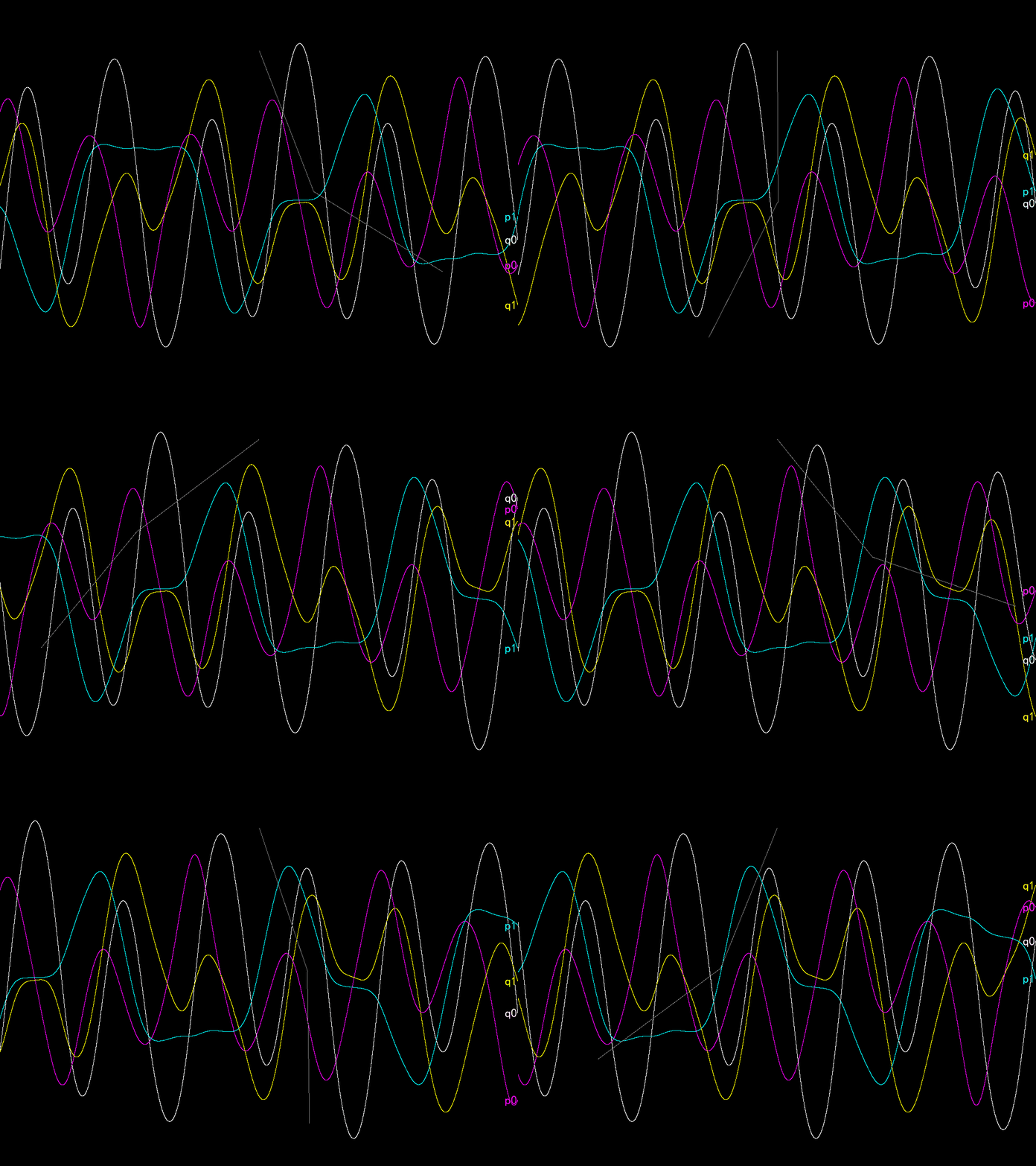
The simulated motion of a double pendulum.

The codes are not complete in this post. See the attached file for details. You can open the project using RPG Maker VX Ace. The Game.exe file is not the official Game.exe executable but the third-party improved version of it called RGD (of version 1.3.2, while the latest till now is 1.5.1).