The longest all-11 substring of a random bit string

Introduction

As a rhythm game player, I often wonder what my max combo will be in my next play. This is a rather unpredictable outcome, and what I can do is to try to conclude a probability distribution of my max combo.

For those who are not familiar with rhythm games and also to make the question clearer, I state the problem in a more mathematical setting.

Consider a random bit string of length $n\in\mathbb N$, where each bit is independent and has probability $Y\in[0,1]$ of being $1$. Let $P_{n,k}(Y)$ be the probability that the length of the longest all-$1$ substring of the bit string is $k\in\mathbb N$ (where obviously $P_{n,k}(Y)$ is nonzero only when $k\le n$). What is the expression of $P_{n,k}(Y)$?

A more interesting problem to consider is what the probability distribution tends to be when $n\to\infty$. Define the random variable $\kappa\coloneqq k/n$ where $k$ is the length of the longest all-$1$ substring. Define a parameter $y\coloneqq Y^n$ (this parameter is held constant while $n\to\infty$). Define the probability distribution function of $\kappa$ as

$$f(y,\kappa)\coloneqq\lim_{n\to\infty}\left(n+1\right)P_{n,\kappa n}\!\left(y^{\frac1n}\right).$$

$$(1)$$

What is the expression of $f(y,\kappa)$?

Notation

Notation for integer range: $a\ldots b$ denotes the integer range defined by the ends $a$ (inclusive) and $b$ (exclusive), or in other words $\left\{a,a+1,\ldots,b-1\right\}$. It is defined to be empty if $a\ge b$. The operator $\ldots$ has a lower precedence than $+$ and $-$ but a higher precedence than $\in$.

The notation $a\,..b$ denotes the inclusive integer range $\left\{a,a+1,\ldots,b\right\}$. It is defined to be empty if $a>b$.

The case for finite $n$

A natural approach to find $P_{n,k}$ is to try to find a recurrence relation of $P_{n,k}$ for different $n$ and $k$, and then use a dynamic programming (DP) algorithm to compute $P_{n,k}$ for any given $n$ and $k$.

The first DP approach

For a rhythm game player, the most straightforward way of finding $k$ for a given bit string is to track the current combo, and update the max combo when the current combo is greater than the previous max combo.

To give the current combo a formal definition, denote each bit in the bit string as $b_i$, where $i\in0\ldots n$. Define the current combo $r_i$ as the length of the longest all-$1$ substring of the bit string ending before (exclusive) $i$ (so $r_i=0$ if $b_{i-1}=0$, which is callled a combo break):

$$r_i\coloneqq\max\left\{r\in0\,..i\,\middle|\,\forall j\in i-r\ldots i:b_j=1\right\},$$

where $i\in0\,..n$.

Now, use three numbers $(n,k,r)$ to define a DP state. Denote $P_{n,k,r}$ to be the probability that the max combo is $k$ and the final combo ($r_n$) is $r$. Then, consider a transition from state $(n,k,r)$ to state $(n+1,k',r')$ by adding a new bit $b_n$ to the bit string. There are two cases:

• If $b_n=0$ (has $1-Y$ probability), then this means a combo break, so we have $r'=0$ and $k'=k$.
• If $b_n=1$ (has $Y$ probability), then the combo continues, so we have $r'=r+1$. The max combo needs to be updated if needed, so we have $k'=\max(k,r')$.

However, in actual implementation of the DP algorithm, we need to reverse this transition by considering what state can lead to the current state $(n,k,r)$ (to use the bottom-up approach).

First, obviously in any possible case $r\in0\,..k$ (currently we only consider the cases where $n>k>0$). Divide all those cases into three groups:

1. If $r=0$, this is means a combo break, so the last bit is $0$, and the previous state can have any possible final combo $r'$. Therefore, it can be transitioned from any $(n-1,k,r')$ where $r'\in0\,..k$. For each possible previous state, the probability of the transition to this new state is $1-Y$.
2. If $r\in1\,..k-1$, this means the last bit is $1$, the previous final combo is $r-1$, and the previous max combo is already $k$. Therefore, the previous state is $(n-1,k,r-1)$, and the probability of the transition is $Y$.
3. If $r=k$, this means the max combo may (or may not) have been updated. In either case, the previous final combo is $r-1=k-1$.

• If the max combo is updated, the previous max combo must be $k-1$ because it must not be less than the previous final combo $k-1$ and must be less than the new max combo $k$. Therefore, the previous state is $(n-1,k-1,k-1)$, and the probability of the transition is $Y$.
• If the max combo is not updated, the previous max combo is the same as the new one, which is $k$. Therefore, the previous state is $(n-1,k,k-1)$, and the probability of the transition is $Y$.

Therefore, we can write a recurrence relation that is valid when $n>k>0$:

$$P_{n,k,r}=\begin{cases} \left(1-Y\right)\sum_{r'=0}^kP_{n-1,k,r'},&r=0\\ YP_{n-1,k,r-1},&r\in1\,..k-1\\ Y\left(P_{n-1,k-1,k-1}+P_{n-1,k,k-1}\right),&r=k. \end{cases}$$

However, there are also other cases (mostly edge cases) because we assumed $n>k>0$. Actually, in the meaningfulness condition $n\ge k\ge r\ge0$ (necessary condition for $P_{n,k,r}$ to be nonzero), there are three inequality that can be altered between a less-than sign or an equal sign, so there are totally $2^3=8$ cases. Considering all those cases (omitted in this article because of the triviality), we can write a recurrence relation that is valid for all $n,k,r$, covering all the edge cases:

$$P_{n,k,r}=\begin{cases} 1,& n=k=r=0,\\ YP_{n-1,n-1,n-1},& n=k=r>0,\\ 0,& n=k>r>0,\\ 0,& n=k>r=0,\\ Y\left(P_{n-1,k-1,k-1}+P_{n-1,k,k-1}\right),& n>k=r>0,\\ YP_{n-1,k,r-1},& n>k>r>0,\\ \left(1-Y\right)\sum_{r'=0}^kP_{n-1,k,r'},& n>k>r=0,\\ \left(1-Y\right)P_{n-1,0,0},& n>k=r=0. \end{cases}$$

$$(2)$$

Note that the probabilities related to note count $n$ only depend on those related to note count $n-1$ and that the probabilities related to max combo $k$ and final combo $r$ only depend on those related to either less max combo than $k$ or less final combo than $r$ (except for the case $n>k>r=0$, which can be specially treated before the current iteration of $k$ actually starts), so for the bottom-up DP we can reduce the spatial complexity from $O\!\left(n^3\right)$ to $O\!\left(n^2\right)$ by reducing the 3-dimensional DP to a 2-dimensional one. What needs to be taken care of is that the DP table needs to be updated from larger $k$ and $r$ to smaller $k$ and $r$ instead of the other way so that the numbers in the last iteration in $n$ are left untouched while we need to use them in the current iteration.

After the final iteration in $n$ finishes, we need to sum over the index $r$ to get the final answer:

$$P_{n,k}=\sum_{r=0}^kP_{n,k,r}.$$

Writing the code for the DP algorithm is then straightforward. Here is an implementation in Ruby. In the code, dp[k][r] means $P_{n,k,r}$ in the $n$th iteration.

1 2 3 4 5 6 7 8 9 10 11 12 13 14

## Returns an array of size m+1, ## with the k-th element being the probability P_{m,k}. def combo m (1..m).each_with_object [[1]] do |n, dp| dp[n] = [0]*n + [Y * dp[n-1][n-1]] # n = k > 0 (n-1).downto 1 do |k| # n > k > 0 dpk0 = (1-Y) * dp[k].sum dp[k][k] = Y * (dp[k-1][k-1] + dp[k][k-1]) # n > k = r > 0 (k-1).downto(1) { |r| dp[k][r] = Y * dp[k][r-1] } # n > k > r > 0 dp[k][0] = dpk0 # n > k > r = 0 end dp[0][0] *= 1-Y # n > k = r = 0 end.map &:sum end

Because of the three nested loops, the time complexity of the DP algorithm is $O\!\left(n^3\right)$.

The second DP approach

Here is an alternative way to use DP to solve the problem. Instead of building a DP table with the $k,r$ indices, we can build a DP table with the $n,k$ indices.

First, we need to rewrite the recurrence relation of $P_{n,k}$ instead of that of $P_{n,k,r}$. We then need to try to express $P_{n,k,r}$ in terms of $P_{n,k}$ terms. The easiest part is the case where $n\ge k=r=0$. By recursively applying Equation 2 to $P_{n,0,0}$, we have

$$\begin{align*} P_{n,0,0}&=\left(1-Y\right)P_{n-1,0,0}\\ &=\left(1-Y\right)^2P_{n-2,0,0}\\ &=\cdots\\ &=\left(1-Y\right)^nP_{0,0,0}. \end{align*}$$

Because $P_{0,0,0}=1$, we have

$$P_{n,0,0}=\left(1-Y\right)^n.$$

$$(3)$$

---

For $n>k>r>0$, we can recursively apply Equation 2 to get

$$\begin{align*} P_{n,k,r}&=YP_{n-1,k,r-1}\\ &=Y^2P_{n-2,k,r-2}\\ &=\cdots \end{align*}$$

This will finally either decend the note count to $k$ or decend the final combo to $0$, determined by which comes first.

• If $n-r\le k$, we will decend to the term $P_{k,k,r-(n-k)}$, which must be zero according to the case $n=k>r=0$ and the case $n=k>r>0$ in Equation 2, so $P_{n,k,r}=0$.
• If $n-r>k$, then we will decend to the term $P_{n-r,k,0}$, which is equal to $\left(1-Y\right)P_{n-r-1,k}$ according to the case $n>k>r=0$ in Equation 2.

Therefore, for $n>k>r>0$, we have

$$P_{n,k,r}=\begin{cases} 0,&n-r\le k,\\ Y^r\left(1-Y\right)P_{n-r-1,k},&n-r>k. \end{cases}$$

$$(4)$$

---

For the case $n>k=r>0$, we can also recursively apply Equation 2 to get

$$\begin{align*} P_{n,k,k}&=Y\left(P_{n-1,k-1,k-1}+P_{n-1,k,k-1}\right)\\ &=Y\left(Y\left(P_{n-2,k-2,k-2}+P_{n-2,k-1,k-2}\right)+P_{n-1,k,k-1}\right)\\ &=\cdots\\ &=Y\left(Y\left(\cdots Y\left(P_{n-k,0,0}+P_{n-k,1,0}\right)+\cdots\right)+P_{n-1,k,k-1}\right)\\ &=Y^kP_{n-k,0,0}+\sum_{j=1}^kY^jP_{n-j,k-j+1,k-j}. \end{align*}$$

We can then substitute Equation 3 and 4 into the above equation. The substitution of Equation 3 can be done without a problem, but the substitution of Equation 4 requires some care because of the different cases.

• If $n-k>k$, then only the case $n-r>k$ in Equation 4 will be involved in the summation.
• If $n-k\le k$, then both cases in Equation 4 will be involved in the summation. To be specific, for $j\in1\,..\,2k-n+1$, we need the case $n-r\le k$ in Equation 4 (where the summed terms are just zero and can be omitted); for other terms in the summation, we need the other case.

Considering both cases, we may realize that we can just modify the range of the summation to $j\in\max(1,2k-n+1)\,..k$ and adopt the case $n-r>k$ in Equation 4 for all terms in the summation. Therefore, we have

$$\begin{align*} P_{n,k,k}&=Y^k\left(1-Y\right)^{n-k}+\sum_{j=\max(1,2k-n+1)}^{k}Y^jY^{k-j}\left(1-Y\right)P_{n-j-(k-j)-1,k-j+1}\\ &=Y^k\left(1-Y\right)^{n-k}+Y^k\left(1-Y\right)\sum_{k'=1}^{\min(k,n-k-1)}P_{n-k-1,k'}, \end{align*}$$

where in the last line we changed the summation index to $k'\coloneqq k-j+1$ to simplify it. Because $P_{n-k-1,0}=P_{n-k-1,0,0}=\left(1-Y\right)^{n-k-1}$ according to Equation 3, we can combine the two terms into one summation to get the final result for $n>k=r>0$:

$$P_{n,k,k}=Y^k\left(1-Y\right)\sum_{k'=0}^{\min(k,n-k-1)}P_{n-k-1,k'}.$$

$$(5)$$

Noticing the obvious fact that $\sum_{k=0}^nP_{n,k}=1$, the above equation can be simplified, when $k\ge n-k-1$, to

$$P_{n,k,k}=Y^k\left(1-Y\right).$$

$$(6)$$

This simplification is not specially useful, but it can be used to simplify the calculation in the program.

---

Then, for $n>k>0$, express $P_{n,k}$ in terms of $P_{n,k,r}$ by summing over $r$, and substitute previous results:

$$\begin{align*} P_{n,k}&=\sum_{r=0}^kP_{n,k,r}\\ &=P_{n,k,0}+P_{n,k,k}+\sum_{r=1}^{k-1}P_{n,k,r}\\ &=\left(1-Y\right)P_{n-1,k}+Y^k\left(1-Y\right)\sum_{k'=0}^{\min(k,n-k-1)}P_{n-k-1,k'}\\ &\phantom{=~}{}+\sum_{r=1}^{\min(k-1,n-k-1)}Y^r\left(1-Y\right)P_{n-r-1,k}\\ &=\left(1-Y\right)\left( Y^k\sum_{k'=0}^{\min(k,n-k-1)}P_{n-k-1,k'} +\sum_{r=0}^{\min(k-1,n-k-1)}Y^rP_{n-r-1,k} \right) \end{align*}$$

where in the last term $r$ is summed to $\min(k-1,n-k-1)$ instead of $k-1$ because of the different cases in Equation 4.

Finally, consider the edge cases where $n=k\ge0$ and $n\ge k=0$ (trivial), we have the complete resursive relation for $P_{n,k}$:

$$P_{n,k}=\begin{cases} Y^n,&n=k\ge0,\\ \left(1-Y\right)^n,&n\ge k=0,\\ \displaystyle{\begin{split} \left(1-Y\right)&\,\left( Y^k\sum_{k'=0}^{\min(k,n-k-1)}P_{n-k-1,k'} \right.\\&\left. +\sum_{r=0}^{\min(k-1,n-k-1)}Y^rP_{n-r-1,k} \right), \end{split}}&n>k>0. \end{cases}$$

$$(7)$$

Then, we can write the program to calculate $P_{n,k}$:

1 2 3 4 5 6 7 8 9 10

## Returns an array of size m+1, ## with the k-th element being the probability P_{m,k}. def combo m (1..m).each_with_object [[1]] do |n, dp| dp[n] = (1..n-1).each_with_object [(1-Y)**n] do |k, dpn| dpn[k] = (1-Y) * (Y**k * (0..[k, n-k-1].min).sum { dp[n-k-1][_1] } + (0..[k-1, n-k-1].min).sum { Y**_1 * dp[n-_1-1][k] }) end dp[n][n] = Y**n end.last end

This algorithm has the same (asymptotic) space and time complexity as the previous one.

Polynomial coefficients

We have wrote programmes to calculate probabilities $P_{n,k}(Y)$ based on given $Y$, which we assumed to be a float number. However, float numbers have limited precision, and the calculation may be inaccurate. Actually, the calculation can be done symbolically.

The probability $P_{n,k}$ is a polynomial of degree (at most) $n$ in $Y$, and the coefficients of the polynomial are integers. This can be easily proven by using mathematical induction and utilizing Equation 7. Therefore, we can calculate the coefficients of the polynomial $P_{n,k}(Y)$ instead of calculate the value directly so that we get a symbolic but accurate result.

Both the two DP algorithms above can be modified to calculate the coefficients of the polynomial. Actually, we can define Y to be a polynomial object that can do arithmetic operations with other polynomials or numbers, and then the programmes can run without any modification. Here, I will modify the second DP algorithm to calculate the coefficients of the polynomial.

We can also utilize Equation 6 to simplify the calculation. Considering the edge cases involved in $\min(k,n-k-1)$ and $\min(k-1,n-k-1)$, there are three cases we need to consider:

1. Case $k>n-k-1$: Equation 6 can be applied, and $r$ is summed to $n-k-1$.
2. Case $k=n-k-1$ (can only happen when $n$ is odd): Equation 6 can be applied, and $r$ is summed to $k-1$.
3. Case $k<n-k-1$: Equation 6 cannot be applied, and $r$ is summed to $k-1$.

Then, use arrays to store the coefficients of the polynomial $P_{n,k}(Y)$, and we can write the program to calculate the coefficients:

1 2 3 4 5 6 7 8 9 10 11 12 13 14 15 16 17 18 19 20 21 22 23 24 25 26 27 28 29 30 31 32 33 34

## Returns a nested array of size m+1 times m+1, ## with the j-th element of the k-th element being the coefficient of Y^j in P_{m,k}(Y). def combo_pc m (1..m).each_with_object [[[1]]] do |n, dp| dp[n] = Array.new(n+1) { Array.new n+1, 0 } # dp[n][0] = (1-Y)**n 0.upto(n-1) { dp[n][0][_1] = dp[n-1][0][_1] } # will be multiplied by 1-Y later 1.upto n/2-1 do |k| # dp[n][k] = (1-Y) * (Y**k * (0..k).sum { |j| dp[n-k-1][j] } + (0..k-1).sum { |r| Y**r * dp[n-r-1][k] }) 0.upto(k) { |j| 0.upto(n-k-1) { dp[n][k][_1+k] += dp[n-k-1][j][_1] } } 0.upto(k-1) { |r| 0.upto(n-r-1) { dp[n][k][_1+r] += dp[n-r-1][k][_1] } } end if n % 2 == 1 k = n/2 # dp[n][k] = (1-Y) * (Y**k + (0..k-1).sum { |r| Y**r * dp[n-r-1][k] }) dp[n][k][k] = 1 0.upto(k-1) { |r| 0.upto(n-r-1) { dp[n][k][_1+r] += dp[n-r-1][k][_1] } } end ((n+1)/2).upto n-1 do |k| # dp[n][k] = (1-Y) * (Y**k + (0..n-k-1).sum { |r| Y**r * dp[n-r-1][k] }) dp[n][k][k] = 1 0.upto(n-k-1) { |r| 0.upto(n-r-1) { dp[n][k][_1+r] += dp[n-r-1][k][_1] } } end 0.upto(n-1) { |k| n.downto(1) { dp[n][k][_1] -= dp[n][k][_1-1] } } # multiply by 1-Y # dp[n][n] = Y**n dp[n][n][n] = 1 end.last end

Here I list first few polynomials $P_{n,k}(Y)$ calculated by the above program:

$$\begin{array}{r|llllc} & k=0 & 1 & 2 & 3 & \cdots\\ \hline n=0 & 1\\ 1 & 1-Y & Y\\ 2 & 1-2Y+Y^2 & 2Y-Y^2 & Y^2\\ 3 & 1-3Y+3Y^2-Y^3 & 3Y-5Y^2+2Y^3 & 2Y^2-2Y^3 & Y^3\\ \vdots \end{array}$$

When evaluating the polynomials for large $n$, the result is inaccurate for $Y$ that is not close to $0$ because of the limited precision of floating numbers. If $Y$ is closer to $1$, we can first find the coefficients of $P_{n,k}(1-X)$ and then substitute $X\coloneqq1-Y$.

Plots of the probability distributions

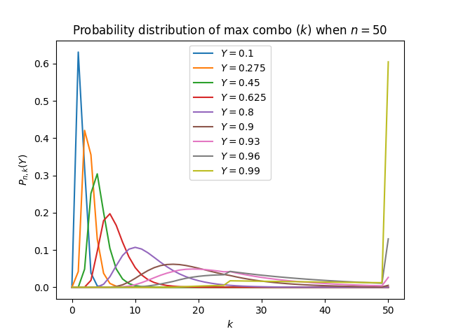
Here are some plots of the probability distribution of max combo $k$ when $n=50$:

n=50

The plots are intuitive as they show that one has higher probability to get a higher max combo when they have a higher success rate.

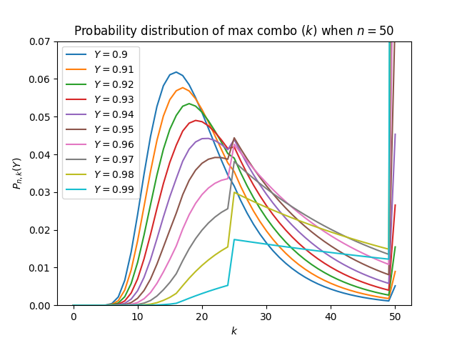
There is a suspicious jump in $P_{n,k}(Y)$ near $k=n/2$ when $Y$ is close to $1$. We can look at it closer:

n=50

In the zoomed-in plot, we can also see a jump in first derivative (w.r.t. $k$) of $P_{n,k}(Y)$ near $k=n/3$. Actually, the jumps can be modeled in later sections when we talk about the case when $n\to\infty$.

The case when $n\to\infty$

A natural approach is to try substituting Equation 7 into Equation 1 to get a function w.r.t. the unknown function $f(y,\kappa)$. First, we can easily write the case when $y=0$ because it means zero success rate, and the only possible max combo is zero:

$$f(y=0,\kappa)=\delta(\kappa).$$

$$(8)$$

Similarly, we can easily write the case when $y=1$:

$$f(y=1,\kappa)=\delta(\kappa-1).$$

$$(9)$$

From now on, we only consider the case when $0<y<1$. First, for the case $\kappa=0$, according to Equation 7,

$$\begin{align*} f(y,\kappa=0)&=\lim_{n\to\infty}\left(n+1\right)\left(1-y^{\frac1n}\right)^n\\ &=\begin{cases}0,&0<y\le1,\\\infty,&y=0.\end{cases} \end{align*}$$

The $\infty$ means that there is a Dirac $\delta$ function (shown in Equation 8).

Then, for the case $\kappa=1$, according to Equation 7,

$$f(y,\kappa=1)=\lim_{n\to\infty}\left(n+1\right)y=\infty.$$

The $\infty$ means that there is a Dirac $\delta$ function. Actually, it is easy to see that there must be a $y\delta(\kappa-1)$ term in the expression of $f(y,\kappa)$ because the probability of getting a max combo ($\kappa=1$) is $y$.

Define

$$h(y,\kappa)\coloneqq f(y,\kappa)-y\delta(\kappa-1),$$

$$(10)$$

and then we can get rid of the infinity here.

From now on, we only consider the case when $0<y<1$ and $0<\kappa<1$. According to Equation 7,

$$\begin{align*} &\phantom{=~}f\!\left(y\in\left(0,1\right),\kappa\in\left(0,1\right)\right)\\ &=\lim_{n\to\infty}\left(n+1\right)\left(1-y^{\frac1n}\right)\left( y^\kappa\sum_{k'=0}^{\min(\kappa n,n-\kappa n-1)}P_{n-\kappa n-1,k'}\!\left(y^{\frac1n}\right) \right.\\&\phantom{=\lim_{n\to\infty}\left(n+1\right)\left(1-y^{\frac1n}\right)}\left. +\sum_{r=0}^{\min(\kappa n-1,n-\kappa n-1)}y^{\frac rn}P_{n-r-1,\kappa n}\!\left(y^{\frac1n}\right) \right)\\ &=\lim_{n\to\infty}n\left(1-y^{\frac1n}\right)\cdot\lim_{n\to\infty}\left( y^\kappa\sum_{t=0,\Delta t=\frac1n}^{\min(\kappa,1-\kappa)}P_{(1-\kappa)n,tn}\!\left(y^{\frac1n}\right) +\sum_{t=0,\Delta t=\frac1n}^{\min(\kappa,1-\kappa)}y^tP_{(1-t)n,\kappa n}\!\left(y^{\frac1n}\right) \right)\\ &=-\ln y\lim_{n\to\infty}\left( y^\kappa\sum_{t=0,\Delta t=\frac1n}^{\min(\kappa,1-\kappa)} \frac1{\left(1-\kappa\right)n}f\!\left(y^{1-\kappa},\frac t{1-\kappa}\right) \right.\\&\phantom{=-\ln y\lim_{n\to\infty}}\left. +\sum_{t=0,\Delta t=\frac1n}^{\min(\kappa,1-\kappa)}y^t \frac1{\left(1-t\right)n}f\!\left(y^{1-t},\frac{\kappa}{1-t}\right) \right)\\ &=-\ln y\lim_{n\to\infty}\sum_{t=0,\Delta t=\frac 1n}^{\min(\kappa,1-\kappa)}\left( \frac{y^\kappa}{1-\kappa}f\!\left(y^{1-\kappa},\frac t{1-\kappa}\right) +\frac{y^t}{1-t}f\!\left(y^{1-t},\frac\kappa{1-t}\right) \right)\Delta t\\ &=-\ln y\int_{t=0}^{\min(\kappa,1-\kappa)}\left( \frac{y^\kappa}{1-\kappa}f\!\left(y^{1-\kappa},\frac t{1-\kappa}\right) +\frac{y^t}{1-t}f\!\left(y^{1-t},\frac\kappa{1-t}\right) \right)\mathrm dt. \end{align*}$$

Add back the delta function at $\kappa=1$, and we have the integral equation

$$\begin{split} f\!\left(y\in\left(0,1\right),\kappa\right)=-\ln y\int_{t=0}^{\min(\kappa,1-\kappa)}&\,\left( \frac{y^\kappa}{1-\kappa}f\!\left(y^{1-\kappa},\frac t{1-\kappa}\right) \right.\\&\left. +\frac{y^t}{1-t}f\!\left(y^{1-t},\frac\kappa{1-t}\right) \right)\mathrm dt+y\delta(\kappa-1). \end{split}$$

There are two terms in the integral. Substitute $u\coloneqq\frac t{1-\kappa}$ in the first term, and we have

$$\begin{align*} \int_{t=0}^{\min\left(\kappa,1-\kappa\right)}\frac{y^\kappa}{1-\kappa}f\!\left(y^{1-\kappa},\frac t{1-\kappa}\right)\mathrm dt &=\int_0^{\min(\frac\kappa{1-\kappa},1)}y^\kappa f\!\left(y^{1-\kappa},u\right)\mathrm du\\ &=\int_0^{\min(\frac\kappa{1-\kappa},1)}\left(y^\kappa h\!\left(y^{1-\kappa},u\right)+y\delta(u-1)\right)\mathrm du. \end{align*}$$

Substitute $v\coloneqq\frac\kappa{1-t}$ in the second term, and we have

$$\begin{align*} \int_{t=0}^{\min(\kappa,1-\kappa)}\frac{y^t}{1-t}f\!\left(y^{1-t},\frac\kappa{1-t}\right)\mathrm dt &=\int_\kappa^{\min\left(\frac\kappa{1-\kappa},1\right)}y^{1-\frac\kappa v}f\!\left(y^{\frac\kappa v},v\right)\frac{\mathrm dv}v\\ &=\int_\kappa^{\min\left(\frac\kappa{1-\kappa},1\right)}\left(y^{1-\frac\kappa v}h\!\left(y^{\frac\kappa v},v\right)+y\delta(v-1)\right)\frac{\mathrm dv}v. \end{align*}$$

Further, let (we only consider $y\in\left(0,1\right)$ from now on)

$$g(y,\kappa)\coloneqq\frac{h(y,\kappa)}{y},$$

$$(11)$$

then the integral equation becomes

$$\begin{split} g(y,\kappa)=-\ln y&\,\left( \int_0^{\min\left(\frac\kappa{1-\kappa},1\right)}\left(g\!\left(y^{1-\kappa},u\right)+\delta(u-1)\right)\mathrm du \right.\\&\left. +\int_\kappa^{\min\left(\frac\kappa{1-\kappa},1\right)}\left(g\!\left(y^{\frac\kappa v},v\right)+\delta(v-1)\right)\frac{\mathrm dv}v \right). \end{split}$$

$$(12)$$

There is another integral equation for $g$. Because $\int_0^1f\!\left(y,\kappa\right)\mathrm d\kappa=1$, we have

$$\int_0^1g\!\left(y,\kappa\right)\mathrm d\kappa=\frac1y-1.$$

$$(13)$$

Equation 12 and 13 are the equations that we are going to utilize to get the expression for $g(y,\kappa)$.

The case $\kappa\in\left(\frac12,1\right)$

In this case, we have

$$\min\!\left(\frac\kappa{1-\kappa},1\right)=1,$$

so the Dirac delta functions in Equation 12 should be considered. In this case, it simplifies to

$$g_1(y,\kappa)\coloneqq g\!\left(y,\kappa\in\left(\frac12,1\right)\right)= -\ln y\left(y^{\kappa-1}+\int_\kappa^1g\!\left(y^{\frac\kappa v},v\right)\frac{\mathrm dv}v+1\right),$$

$$(14)$$

where Equation 13 is utilized when finding the first term. We can try to solve Equation 14 by using Adomian decomposition method (ADM). Suppose $g_1$ can be written in a series

$$g_1=g_1^{(0)}+g_1^{(1)}+\cdots,$$

and substitute it into Equation 14, and we have

$$g_1^{(0)}(y,\kappa)+\cdots =-\ln y\left(y^{\kappa-1}+1+\int_\kappa^1\left( g^{(0)}\!\left(y^{\frac\kappa v},v\right)+\cdots \right)\frac{\mathrm dv}v\right).$$

Assume we may interchange integration and summation (which is OK here because we can verify the solution after we find it using ADM). Then,

$$\begin{align*} &\phantom{=~}g_1^{(0)}(y,\kappa)+g_1^{(1)}(y,\kappa)+\cdots\\ &=-\ln y\left(y^{\kappa-1}+1\right) -\ln y\int_\kappa^1g^{(0)}\!\left(y^{\frac\kappa v},v\right)\frac{\mathrm dv}v-\cdots. \end{align*}$$

If we let

$$\begin{split} g_1^{(0)}(y,\kappa)&\coloneqq-\ln y\left(y^{\kappa-1}+1\right),\\ g_1^{(i+1)}(y,\kappa)&\coloneqq-\ln y\int_\kappa^1g^{(i)}\!\left(y^{\frac\kappa v},v\right)\frac{\mathrm dv}v,\quad i\in\mathbb N, \end{split}$$

$$(15)$$

then we can equate each term in the two series. If the sum $g_1=\sum_{i=0}^\infty g_1^{(i)}$ converges, then this is a guess of the solution to Equation 14, which we can verify whether it is correct or not.

Using Equation 15, we can find first few terms in the series by directly integrating. The first few terms are

$$\begin{split} g_1^{(0)}(y,\kappa)&=-\ln y\left(y^{\kappa-1}+1\right),\\ g_1^{(1)}(y,\kappa)&=-\ln y\left(y^{\kappa-1}-1+\ln y^{\kappa-1}\right),\\ g_1^{(2)}(y,\kappa)&=-\ln y\left(y^{\kappa-1}-1-\ln y^{\kappa-1}+\frac12\left(\ln y^{\kappa-1}\right)^2\right),\\ g_1^{(3)}(y,\kappa)&=-\ln y\left(y^{\kappa-1}-1-\ln y^{\kappa-1}-\frac12\left(\ln y^{\kappa-1}\right)^2+\frac16\left(\ln y^{\kappa-1}\right)^3\right),\\ \vdots& \end{split}$$

We may then guess that the terms have general formula

$$g_1^{(i)}(y,\kappa)=-\ln y\left(y^{\kappa-1}+\frac1{i!}\left(\ln y^{\kappa-1}\right)^i -\sum_{j=0}^{i-1}\frac1{j!}\left(\ln y^{\kappa-1}\right)^j\right).$$

Sum up the terms, and we have $$\begin{align*} g_1(y,\kappa)&=\sum_{i=0}^\infty g_1^{(i)}(y,\kappa)\\ &=\lim_{q\to\infty}\sum_{i=0}^q-\ln y\left( y^{\kappa-1}+\frac1{i!}\left(\ln y^{\kappa-1}\right)^i -\sum_{j=0}^{i-1}\frac1{j!}\left(\ln y^{\kappa-1}\right)^j \right)\\ &=-\ln y\left(\exp\ln y^{\kappa-1}+\lim_{q\to\infty}\left( \left(q+1\right)y^{\kappa-1} -\sum_{j=0}^q\sum_{i=j+1}^q\frac1{j!}\left(\ln y^{\kappa-1}\right)^j \right)\right)\\ &=-\ln y\left(y^{\kappa-1}+\lim_{q\to\infty}\left( \left(q+1\right)y^{\kappa-1} -\sum_{j=0}^q\frac{q-j}{j!}\left(\ln y^{\kappa-1}\right)^j \right)\right)\\ &=-\ln y\left( y^{\kappa-1}+\lim_{q\to\infty}\left( qy^{\kappa-1}-q\sum_{j=0}^q\frac1{j!}\left(\ln y^{\kappa-1}\right)^j \right) \right.\\&\phantom{=-\ln y}\left.\vphantom{\sum_j^q} +y^{\kappa-1} +\ln y^{\kappa-1}\exp\ln y^{\kappa-1} \right)\\ &=-\ln y\left(2+\ln y^{\kappa-1}\right)y^{\kappa-1}. \end{align*}$$

Therefore, we have the final guess of solution

$$g_1(y,\kappa)=-\ln y\left(2+\ln y^{\kappa-1}\right)y^{\kappa-1}.$$

$$(16)$$

We can substitute it into Equation 14 to verify that it is indeed the solution.

The case $\kappa\in\left(\frac13,\frac12\right)$

In this case, we have

$$\min\!\left(\frac\kappa{1-\kappa},1\right)=\frac\kappa{1-\kappa}\in\left(\frac12,1\right).$$

We can then use the same method as in the previous case to find the solution. First, by Equation 14,

$$\begin{align*} g_2(y,\kappa)&\coloneqq g\!\left(y,\kappa\in\left(\frac13,\frac12\right)\right)\\ &=-\ln y\left( \int_0^{\frac\kappa{1-\kappa}}g\!\left(y^{1-\kappa},u\right)\mathrm du +\int_\kappa^{\frac\kappa{1-\kappa}}g\!\left(y^{\frac\kappa v},v\right)\frac{\mathrm dv}v \right)\\ &=-\ln y\left( \int_0^1g\!\left(y^{1-\kappa},u\right)\mathrm du -\int_{\frac\kappa{1-\kappa}}^1g_1\!\left(y^{1-\kappa},u\right)\mathrm du \right.\\&\phantom{=-\ln y}\left. +\int_\kappa^{\frac12}g_2\!\left(y^{\frac\kappa v},v\right)\frac{\mathrm dv}v +\int_{\frac12}^{\frac\kappa{1-\kappa}}g_1\!\left(y^{\frac\kappa v},v\right)\frac{\mathrm dv}v \right). \end{align*}$$

Substitute Equation 13 and 16 into the above equation, and we have

$$\begin{split} g_2(y,\kappa)&=-\ln y\left( y^{\kappa-1} +y^{-\kappa}\left(1+\ln y^{-\kappa}\right) -2y^{2\kappa-1}\left(1+\ln y^{2\kappa-1}\right) \vphantom{\int_\kappa^{\frac12}}\right.\\&\phantom{=-\ln y}\left. +\int_\kappa^{\frac12}g_2\!\left(y^{\frac\kappa v},v\right)\frac{\mathrm dv}v \right). \end{split}$$

$$(17)$$

Equation 17 can again be solved by ADM though the calculation is much more complicated than the previous case. We may guess $g_2=\sum_{i=0}^\infty g_2^{(i)}$ is the solution if the series converges, where

$$\begin{split} g_2^{(0)}(y,\kappa)&\coloneqq-\ln y\left( y^{\kappa-1} +y^{-\kappa}\left(1+\ln y^{-\kappa}\right) -2y^{2\kappa-1}\left(1+\ln y^{2\kappa-1}\right) \right),\\ g_1^{(i+1)}(y,\kappa)&\coloneqq-\ln y\int_\kappa^{\frac12}g^{(i)}\!\left(y^{\frac\kappa v},v\right)\frac{\mathrm dv}v, \quad i\in\mathbb N. \end{split}$$

The first few terms go too long to be written here before one may find the pattern, so they are omitted here. If you want to see them, use a mathematical software to help you, and you should be able to find the pattern after calculating first six (or so) terms. After looking at first few terms, the guessed general term is

$$\begin{align*} g_2^{(i)}=-\ln y&\,\left( y^{\kappa-1}+2y^{2\kappa-1}\left(i-1-\ln y^{2\kappa-1}\right) -2\sum_{j=0}^{i-1}\frac{i-j-1}{j!}\left(\ln y^{2\kappa-1}\right)^j \right.\\&\left. {}-y^{-\kappa}\sum_{j=0}^{i-1}\frac1{j!}\left(\ln y^{2\kappa-1}\right)^j +\frac1{i!}y^{-\kappa}\left(1+\ln y^{-\kappa}\right)\left(\ln y^{2\kappa-1}\right)^i \right). \end{align*}$$

Then we can sum it to get a guess of $g_2$. After some tedious calculation, we have

$$g_2(y,\kappa)=-\ln y\left( \left(2+\ln y^{\kappa-1}\right)y^{\kappa-1} -\left(2+4\ln y^{2\kappa-1}+\left(\ln y^{2\kappa-1}\right)^2\right)y^{2\kappa-1} \right).$$

$$(18)$$

On may verify that this is indeed the solution by substituting it into Equation 17.

The case $\kappa\in\left(\frac14,\frac13\right)$

By using very similar methods but after very tedious calculation, the solution is

$$\begin{split} g_3(y,\kappa)&\coloneqq g\!\left(y,\kappa\in\left(\frac14,\frac13\right)\right)\\ &=-\ln y\left( \left(2+\ln y^{\kappa-1}\right)y^{\kappa-1} -\left(2+4\ln y^{2\kappa-1}+\left(\ln y^{2\kappa-1}\right)^2\right)y^{2\kappa-1}\vphantom{\frac12} \right.\\&\phantom{=-\ln y}\left. {}+\left(3\ln y^{3\kappa-1}+3\left(\ln y^{3\kappa-1}\right)^2+\frac12\left(\ln y^{3\kappa-1}\right)^3\right)y^{3\kappa-1} \right). \end{split}$$

$$(19)$$

Other cases

After seeing Equation 16, 18, and 19, one may guess the form of solution for other cases.

Guess the form of solution for $\kappa\in\left(\frac1{q+1},\frac1q\right)$, where $q\in1\ldots\infty$, is

$$g_q(y,\kappa)\coloneqq g\!\left(y,\kappa\in\left(\frac1q,\frac1{q+1}\right)\right)=\sum_{s=1}^q\Delta g_s(y,\kappa),$$

where

$$\Delta g_s(y,\kappa)\coloneqq\left(-1\right)^sy^{s\kappa-1}\ln y\sum_{j=0}^s\frac{A_{s,j}}{j!}\left(\ln y^{s\kappa-1}\right)^j,$$

where $A_{s,j}$ are coefficients to be determined.

Now, consider the cases $q\in2\ldots\infty$. Because $\kappa\in\left(\frac1{q+1},\frac1q\right)$,

$$\min\!\left(\frac\kappa{1-\kappa},1\right)=\frac\kappa{1-\kappa}\in\left(\frac1q,\frac1{q-1}\right).$$

Therefore,

$$\begin{align*} &\phantom{=~}\int_0^{\min\left(\frac\kappa{1-\kappa},1\right)}\left(g\!\left(y^{1-\kappa},u\right)+\delta(u-1)\right)\mathrm du\\ &=\int_0^1g\!\left(y^{1-\kappa},u\right)\mathrm du -\sum_{p=1}^{q-2}\int_{\frac1{p+1}}^{\frac1p}g_p\!\left(y^{1-\kappa},u\right)\mathrm du -\int_{\frac\kappa{1-\kappa}}^\frac1{q-1}g_{q-1}\!\left(y^{1-\kappa},u\right)\mathrm du\\ &=y^{\kappa-1}-1 -\sum_{p=1}^{q-2}\int_{\frac1{p+1}}^{\frac1p}\sum_{s=1}^p\Delta g_s\!\left(y^{1-\kappa},u\right)\mathrm du -\int_{\frac\kappa{1-\kappa}}^\frac1{q-1}\sum_{s=1}^{q-1}\Delta g_s\!\left(y^{1-\kappa},u\right)\mathrm du\\ &=y^{\kappa-1}-1 -\sum_{s=1}^{q-1}\left( \sum_{p=s}^{q-2}\int_{\frac1{p+1}}^{\frac1p}+\int_{\frac\kappa{1-\kappa}}^\frac1{q-1} \right)\Delta g_s\!\left(y^{1-\kappa},u\right)\mathrm du\\ &=y^{\kappa-1}-1 -\sum_{s=1}^{q-1}\int_{\frac\kappa{1-\kappa}}^{\frac1s}\Delta g_s\!\left(y^{1-\kappa},u\right)\mathrm du, \end{align*}$$

and

$$\begin{align*} &\phantom{=~}\int_\kappa^{\min\left(\frac\kappa{1-\kappa},1\right)}\left(g\!\left(y^{\frac\kappa v},v\right)+\delta(v-1)\right)\frac{\mathrm dv}v\\ &=\int_\kappa^{\frac1q}g_q\!\left(y^{\frac\kappa v},v\right)\frac{\mathrm dv}v +\int_{\frac1q}^{\frac\kappa{1-\kappa}}g_{q-1}\!\left(y^{\frac\kappa v},v\right)\frac{\mathrm dv}v\\ &=\int_\kappa^{\frac1q}\sum_{s=1}^q\Delta g_s\!\left(y^{\frac\kappa v},v\right)\frac{\mathrm dv}v +\int_{\frac1q}^{\frac\kappa{1-\kappa}}\sum_{s=1}^{q-1}\Delta g_s\!\left(y^{\frac\kappa v},v\right)\frac{\mathrm dv}v\\ &=\sum_{s=1}^{q-1}\int_\kappa^{\frac\kappa{1-\kappa}}\Delta g_s\!\left(y^{\frac\kappa v},v\right)\frac{\mathrm dv}v +\int_\kappa^{\frac1q}\Delta g_q\!\left(y^{\frac\kappa v},v\right)\frac{\mathrm dv}v. \end{align*}$$

Substitute into Equation 12, and we have

$$\begin{split} \sum_{s=1}^q\Delta g_s(y,\kappa)=-\ln y&\,\left( y^{\kappa-1}-1 -\sum_{s=1}^{q-1}\int_{\frac\kappa{1-\kappa}}^{\frac1s}\Delta g_s\!\left(y^{1-\kappa},u\right)\mathrm du \right.\\&\left. {}+\sum_{s=1}^{q-1}\int_\kappa^{\frac\kappa{1-\kappa}}\Delta g_s\!\left(y^{\frac\kappa v},v\right)\frac{\mathrm dv}v +\int_\kappa^{\frac1q}\Delta g_q\!\left(y^{\frac\kappa v},v\right)\frac{\mathrm dv}v \right). \end{split}$$

$$(20)$$

To simplify later expressions, define

$$B_{s,l}\coloneqq\left(-1\right)^l\sum_{j=l}^s\left(-1\right)^jA_{s,j}.$$

$$(21)$$

Now, calculate the integrals in Equation 20. Before that, first we introduce a handy integral formula:

$$\int\left(\ln w\right)^j\,\mathrm dw =\left(-1\right)^jj!\,w\sum_{l=0}^j\left(-1\right)^l\frac{\left(\ln w\right)^l}{l!}+C.$$

This formula can be proved by mathematical induction and integration by parts.

Then, we have

$$\begin{align*} &\phantom{=~}\int_{\frac\kappa{1-\kappa}}^{\frac1s}\Delta g_s\!\left(y^{1-\kappa},u\right)\mathrm du\\ &=\int_{\frac\kappa{1-\kappa}}^{\frac1s}\left(-1\right)^s y^{\left(su-1\right)\left(1-\kappa\right)}\ln y^{1-\kappa} \sum_{j=0}^s\frac{A_{s,j}}{j!}\left(\ln y^{\left(su-1\right)\left(1-\kappa\right)}\right)^j\,\mathrm du\\ &=\frac{\left(-1\right)^s}s\sum_{j=0}^s\frac{A_{s,j}}{j!} \int_{\frac\kappa{1-\kappa}}^{\frac1s}\left(\ln y^{\left(su-1\right)\left(1-\kappa\right)}\right)^j\, \mathrm d\left(\ln y^{\left(su-1\right)\left(1-\kappa\right)}\right)\\ &=\frac{\left(-1\right)^s}s\sum_{j=0}^s\frac{A_{s,j}}{j!} \int_{y^{\left(s+1\right)\kappa-1}}^1\left(\ln w\right)^j\,\mathrm dw\\ &=\frac{\left(-1\right)^s}s\sum_{j=0}^s\frac{A_{s,j}}{j!} \left(-1\right)^jj!\left( 1 -y^{\left(s+1\right)\kappa-1} \sum_{l=0}^j\left(-1\right)^l\frac{\left(\ln y^{\left(s+1\right)\kappa-1}\right)^l}{l!} \right)\\ &=\frac{\left(-1\right)^s}s\sum_{j=0}^s\left(-1\right)^jA_{s,j} -\frac{\left(-1\right)^s}sy^{\left(s+1\right)\kappa-1} \sum_{l=0}^s\left(-1\right)^l\frac{\left(\ln y^{\left(s+1\right)\kappa-1}\right)^l}{l!} \sum_{j=l}^s\left(-1\right)^jA_{s,j}\\ &=\left(-1\right)^s\left( \frac{B_{s,0}}s -\frac1sy^{\left(s+1\right)\kappa-1} \sum_{l=0}^s\frac{B_{s,l}}{l!} \left(\ln y^{\left(s+1\right)\kappa-1}\right)^l \right). \end{align*}$$

$$\begin{align*} &\phantom{=~}\int_\kappa^{\frac\kappa{1-\kappa}}\Delta g_s\!\left(y^{\frac\kappa v},v\right)\frac{\mathrm dv}v\\ &=\int_\kappa^{\frac\kappa{1-\kappa}}\left(-1\right)^s y^{\frac\kappa v\left(sv-1\right)}\ln y^{\frac\kappa v} \sum_{j=0}^s\frac{A_{s,j}}{j!}\left(\ln y^{\frac\kappa v\left(sv-1\right)}\right)^j\frac{\mathrm dv}v\\ &=\left(-1\right)^s\sum_{j=0}^s\frac{A_{s,j}}{j!} \int_\kappa^{\frac\kappa{1-\kappa}}\left(\ln y^{\frac\kappa v\left(sv-1\right)}\right)^j\, \mathrm d\left(\ln y^{\frac\kappa v\left(sv-1\right)}\right)\\ &=\left(-1\right)^s\sum_{j=0}^s\frac{A_{s,j}}{j!} \int_{y^{s\kappa-1}}^{y^{\left(s+1\right)\kappa-1}}\left(\ln w\right)^j\,\mathrm dw\\ &=\left(-1\right)^s\sum_{j=0}^s\frac{A_{s,j}}{j!}\left(-1\right)^jj!\left( y^{\left(s+1\right)\kappa-1}\sum_{l=0}^j\left(-1\right)^l\frac{\left(\ln y^{\left(s+1\right)\kappa-1}\right)^l}{l!} \right.\\&\phantom{=\left(-1\right)^s\sum_{j=0}^s\frac{A_{s,j}}{j!}\left(-1\right)^jj!}\left. {}-y^{s\kappa-1}\sum_{l=0}^j\left(-1\right)^l\frac{\left(\ln y^{s\kappa-1}\right)^l}{l!} \right)\\ &=\left(-1\right)^s\left( y^{\left(s+1\right)\kappa-1}\sum_{l=0}^s\frac{B_{s,l}}{l!} \left(\ln y^{\left(s+1\right)\kappa-1}\right)^l -y^{s\kappa-1}\sum_{l=0}^s\frac{B_{s,l}}{l!} \left(\ln y^{s\kappa-1}\right)^l \right). \end{align*}$$

$$\begin{align*} &\phantom{=~}\int_\kappa^{\frac1q}\Delta g_q\!\left(y^{\frac\kappa v},v\right)\frac{\mathrm dv}v\\ &=\left(-1\right)^q\left( B_{q,0} -y^{q\kappa-1}\sum_{l=0}^q\frac{B_{q,l}}{l!}\left(\ln y^{q\kappa-1}\right)^l \right). \end{align*}$$

Substitute these results into Equation 20, and we have

$$\begin{split} &\phantom{=~}\sum_{s=1}^q \left(-1\right)^sy^{s\kappa-1}\ln y\sum_{j=0}^s\frac{A_{s,j}}{j!}\left(\ln y^{s\kappa-1}\right)^j\\ &=-\ln y\left(\vphantom{\sum_l^s} y^{\kappa-1}-1 \right.\\&\phantom{=-\ln y}\left. {}-\sum_{s=1}^{q-1}\left(-1\right)^s\left( \frac{B_{s,0}}s -\frac1sy^{\left(s+1\right)\kappa-1} \sum_{l=0}^s\frac{B_{s,l}}{l!} \left(\ln y^{\left(s+1\right)\kappa-1}\right)^l \right) \right.\\&\phantom{=-\ln y}\left. {}+\sum_{s=1}^{q-1}\left(-1\right)^s\left( y^{\left(s+1\right)\kappa-1}\sum_{l=0}^s\frac{B_{s,l}}{l!} \left(\ln y^{\left(s+1\right)\kappa-1}\right)^l -y^{s\kappa-1}\sum_{l=0}^s\frac{B_{s,l}}{l!} \left(\ln y^{s\kappa-1}\right)^l \right) \right.\\&\phantom{=-\ln y}\left. {}+\left(-1\right)^q\left( B_{q,0} -y^{q\kappa-1}\sum_{l=0}^q\frac{B_{q,l}}{l!}\left(\ln y^{q\kappa-1}\right)^l \right) \right). \end{split}$$

Cancel factor $\ln y$ on both sides, and we have

$$\begin{align*} &\phantom{=~}\sum_{s=1}^q \left(-1\right)^sy^{s\kappa-1}\sum_{j=0}^s\frac{A_{s,j}}{j!}\left(\ln y^{s\kappa-1}\right)^j\\ &=-y^{\kappa-1}+1\\ &\phantom{=}{}+\sum_{s=1}^{q-1}\left(-1\right)^s\frac{B_{s,0}}s -\sum_{s=2}^q\frac{\left(-1\right)^{s-1}}{s-1}y^{s\kappa-1}\sum_{l=0}^{s-1}B_{s-1,l}\frac{\left(\ln y^{s\kappa-1}\right)^l}{l!}\\ &\phantom{=}{}-\sum_{s=2}^q\left(-1\right)^{s-1}y^{s\kappa-1}\sum_{l=0}^{s-1}B_{s-1,l}\frac{\left(\ln y^{s\kappa-1}\right)^l}{l!} +\sum_{s=1}^{q-1}\left(-1\right)^sy^{s\kappa-1}\sum_{l=0}^sB_{s,l}\frac{\left(\ln y^{s\kappa-1}\right)^l}{l!}\\ &\phantom{=}{}-\left(-1\right)^qB_{q,0}+\left(-1\right)^qy^{q\kappa-1}\sum_{l=0}^qB_{q,l}\frac{\left(\ln y^{q\kappa-1}\right)^l}{l!}\\ &=1+\sum_{s=1}^{q-1}\frac{\left(-1\right)^s}sB_{s,0}-\left(-1\right)^qB_{q,0}&(*)\\ &\phantom{=}-y^{\kappa-1}\left(1+B_{1,0}-B_{1,1}\ln y^{\kappa-1}\right)&(**)\\ &\phantom{=}{}+\sum_{s=2}^q\left(-1\right)^sy^{s\kappa-1}\left( \sum_{l=0}^{s-1}\left(\frac s{s-1}B_{s-1,l}+B_{s,l}\right)\frac{\left(\ln y^{s\kappa-1}\right)^l}{l!} +B_{s,s}\frac{\left(\ln y^{s\kappa-1}\right)^s}{s!} \right)&(***) \end{align*}$$

Equate the coefficients in Line (*) with the corresponding ones on the LHS, and we have

$$0=1+\sum_{s=1}^{q-1}\frac{\left(-1\right)^s}sB_{s,0}-\left(-1\right)^qB_{q,0}.$$

This equation holds for any $q\in 2\ldots\infty$, so

$$\begin{cases} \left(-1\right)^qB_{q,0}=1+\sum_{s=1}^{q-1}\frac{\left(-1\right)^s}sB_{s,0},\\ \left(-1\right)^{q+1}B_{q+1,0}=1+\sum_{s=1}^{q}\frac{\left(-1\right)^s}sB_{s,0}, \end{cases}\quad q\in 2\ldots\infty.$$

Subtract the two equations, and we have

$$B_{q+1,0}=-\frac{q+1}qB_{q,0},\quad q\in 2\ldots\infty.$$

$$(22)$$

Equation 22 can determine $B_{q,0}$ for all $q\in 2\ldots\infty$ once $B_{2,0}$ is determined. The relationship between $B_{1,0}$ and $B_{2,0}$ cannot be described by Equation 22, but is given by

$$B_{2,0}=1-B_{1,0}.$$

$$(23)$$

Equate the coefficients in Line (**) with the corresponding ones on the LHS, and we have

$$A_{1,0}=1+B_{1,0},\quad A_{1,1}=B_{1,1}.$$

By Equation 21, this is equivalent to

$$A_{1,0}=1+A_{1,0}-A_{1,1},\quad A_{1,1}=A_{1,1}.$$

Therefore, $A_{1,1}=1$, and thus

$$B_{1,1}=1.$$

$$(24)$$

Equate the coefficients in Line (***) with the corresponding ones on the LHS, and we have

$$A_{s,l}=\frac s{s-1}B_{s-1,l}+B_{s,l},\quad A_{s,s}=B_{s,s}.$$

By Equation 21, $B_{s,l}=A_{s,l}-B_{s,l+1}$ for $l\in 0\ldots s$, and $A_{s,s}=B_{s,s}$ is always true. Therefore,

$$0=\frac s{s-1}B_{s-1,l}-B_{s,l+1}.$$

This equation is true for any $s\in 2\,..q$ and $l\in0\ldots s$. Because $q$ is arbitrary, we can change the variable $s$ to $q$ and the equation tells us exactly the same information. Therefore,

$$B_{q,l}=\frac q{q-1}B_{q-1,l-1},\quad q\in 2\ldots\infty,\quad l\in 1\,..q.$$

$$(25)$$

Equation 22, 23, 24, and 25 are sufficient to determine $B_{q,l}$ for all $q\in 1\ldots\infty$ and $l\in 0\,..q$ up to one arbitrary parameter. Define the arbitrary parameter

$$b\coloneqq1-B_{1,0},$$

then the first few $B_{q,l}$ are

$$\begin{array}{r|ccccc} &k=0&1&2&3&4\\ \hline q=1&1-b&1\\ 2&2b&2-2b&2\\ 3&-3b&3b&3-3b&3\\ 4&4b&-4b&4b&4-4b&4\\ \vdots&\ddots \end{array}$$

The general formula for $B_{q,l}$ is

$$B_{q,l}=\begin{cases} q,&l=q,\\ q\left(1-b\right),&l=q-1,\\ \left(-1\right)^{q+l}qb,&l\in 0\,..q-2, \end{cases}$$

which may be proved by mathematical induction.

Actually, one may find $b=0$ by simply comparing with the results in Equation 16, 18, or 19. Another way to find $b$ is comparing with Eqution 13. Here I wil show the latter approach.

$$\begin{align*} &\phantom{=~}\int_0^1g\!\left(y,\kappa\right)\mathrm d\kappa\\ &=\sum_{q=1}^\infty\int_{\frac1{q+1}}^{\frac1q}g_q\!\left(y,\kappa\right)\mathrm d\kappa\\ &=\sum_{q=1}^\infty\int_{\frac1{q+1}}^{\frac1q}\sum_{s=1}^q\Delta g_s\!\left(y,\kappa\right)\mathrm d\kappa\\ &=\sum_{s=1}^\infty\sum_{q=s}^\infty\int_{\frac1{q+1}}^{\frac1q}\Delta g_s\!\left(y,\kappa\right)\mathrm d\kappa\\ &=\sum_{s=1}^\infty\int_0^{\frac1s}\Delta g_s\!\left(y,\kappa\right)\mathrm d\kappa\\ &=\sum_{s=1}^\infty\int_0^{\frac1s}\left(-1\right)^sy^{s\kappa-1}\ln y \sum_{j=0}^s\frac{A_{s,j}}{j!}\left(\ln y^{s\kappa-1}\right)^j\,\mathrm d\kappa\\ &=\sum_{s=1}^\infty\frac{\left(-1\right)^s}s\sum_{j=0}^s\frac{A_{s,j}}{j!} \int_0^{\frac1s}\left(\ln y^{s\kappa-1}\right)^j\,\mathrm d\left(y^{s\kappa-1}\right)\\ &=\sum_{s=1}^\infty\frac{\left(-1\right)^s}s\left( B_{s,0}-y^{-1}\sum_{l=0}^sB_{s,l}\frac{\left(\ln y\right)^l}{l!} \right)\\ &=-\left(1-b\right)+y^{-1}\left(\left(1-b\right)-\ln y\right)\\ &\phantom{=}{}+\sum_{s=2}^\infty\frac{\left(-1\right)^s}s\left( \left(-1\right)^ssb-y^{-1}\left( \sum_{l=0}^{s-2}\left(-1\right)^{s+l}sb\frac{\left(\ln y\right)^l}{l!} \right.\right.\\&\phantom{ ={}+\sum_{s=2}^\infty\frac{\left(-1\right)^s}s~\left(\vphantom{\sum_s^\infty}\right.\left(-1\right)^ssb-y^{-1} }\left.\left. {}+s\left(1-b\right)\frac{\left(-\ln y\right)^{s-1}}{\left(s-1\right)!} +s\frac{\left(-\ln y\right)^s}{s!} \right) \right)\\ &=b-1+y^{-1}\left(1-b-\ln y\right) +y^{-1}\sum_{s=2}^\infty\left(\frac{\left(\ln y\right)^{s-1}}{\left(s-1\right)!}-\frac{\left(\ln y\right)^s}{s!}\right)\\ &\phantom{=}{}+b\sum_{s=2}^\infty\left(1-y^{-1}\sum_{l=0}^{s-1}\frac{\left(\ln y\right)^l}{l!}\right)\\ &=b-1+y^{-1}\left(1-b-\ln y\right)+y^{-1}\left(\left(\exp\ln y-1\right)-\left(\exp\ln y-\ln y-1\right)\right)\\ &\phantom{=}{}+b\lim_{q\to\infty}\sum_{s=2}^q\left(1-y^{-1}\sum_{l=0}^{s-1}\left(\ln y\right)^l\right)\\ &=b-1+y^{-1}\left(1-b\right) +b\lim_{q\to\infty}\left(q-1-y^{-1}\left(q-1+\sum_{l=1}^{q-1}\frac{q-l}{l!}\left(\ln y\right)^l\right)\right)\\ &=b-1+y^{-1}\left(1-b\right)+b\left(-1+y^{-1}+\ln y\right)\\ &=y^{-1}-1+b\ln y. \end{align*}$$

Compare the result with Equation 13, we have

$$b=0.$$

The table of $B_{q,l}$ is now

$$\begin{array}{r|ccccc} &k=0&1&2&3&4\\ \hline q=1&1&1\\ 2&0&2&2\\ 3&0&0&3&3\\ 4&0&0&0&4&4\\ \vdots&\ddots \end{array}$$

The table of $A_{s,j}$ is then

$$\begin{array}{r|ccccc} &j=0&1&2&3&4\\ \hline s=1&2&1\\ 2&2&4&2\\ 3&0&3&6&3\\ 4&0&0&4&8&4\\ \vdots&\ddots \end{array}$$

The general formula for $A_{s,j}$ is

$$A_{s,j}=\begin{cases} s,&j\in\left\{s,s-2\right\},\\ 2s,&j=s-1,\\ 0,&j\in0\,..s-3. \end{cases}$$

$$(26)$$

Therefore, the functions $\Delta g_s$ are

$$\Delta g_s(y,\kappa)=\begin{cases} -y^{\kappa-1}\ln y\left(2+\ln y^{\kappa-1}\right),&s=1\\ \begin{split} &\textstyle{\frac{s\left(-1\right)^s}{\left(s-2\right)!}y^{s\kappa-1}\ln y\left(\ln y^{s\kappa-1}\right)^{s-2} \left(1\vphantom{\left(\ln y^{s\kappa-1}\right)^2}\right.}\\ &\textstyle{\left.\quad{}+\frac2{s-1}\ln y^{s\kappa-1}+\frac1{s\left(s-1\right)}\left(\ln y^{s\kappa-1}\right)^2\right),} \end{split}&s\in2\ldots\infty. \end{cases}$$

Therefore, the functions $g_q$ are

$$\begin{split} &g_q(y,\kappa)=-y^{\kappa-1}\ln y\left(2+\ln y^{\kappa-1}\right) +\ln y\sum_{s=2}^q\frac{s\left(-1\right)^s}{\left(s-2\right)!}y^{s\kappa-1}\left(\ln y^{s\kappa-1}\right)^{s-2} \left(1\vphantom{\frac{\left(-1\right)^s}{s!}}\right.\\ &\phantom{g_q(y,\kappa)=\quad}\left.{}+\frac2{s-1}\ln y^{s\kappa-1}+\frac1{s\left(s-1\right)}\left(\ln y^{s\kappa-1}\right)^2\right) \end{split}$$

$$(27)$$

(the formula is also applicable to $q=1$).

Edge cases

Now we have covered almost all cases. The only cases that we have not covered are the cases when $\kappa=\frac1q$, where $q\in2\ldots\infty$. The discontinuity in $g$ at $\kappa=\frac1q$ is

$$\begin{split} &\phantom{=~}g\!\left(y,\frac1q^+\right)-g\!\left(y,\frac1q^-\right)\\ &=-\Delta g_q\!\left(y,\frac1q\right)\\ &=\begin{cases} -2\ln y,&q=2,\\ 0,&q\in3\ldots\infty. \end{cases} \end{split}$$

$$(28)$$

Therefore, for $q\in3\ldots\infty$, the function $g$ has defined limit at $\kappa=\frac1q$, and the value of $g$ here should just be the limit value. Now, the only problem is at $\kappa=\frac12$. We should determine whether the value of $g$ at $\kappa=\frac12$ is its left limit or right limit.

Looking at Equation 12, one may see that the discontinuity at $\kappa=\frac12$ is due to the Dirac $\delta$ function in the integrand. Therefore, whether $g$ at $\kappa=\frac12$ is $g_1$ or $g_2$ depends on whether the Dirac $\delta$ function is within the integrated interval. If it is, then $g$ at $\kappa=\frac12$ is $g_1$; otherwise, it is $g_2$.

The inclusion of the Dirac $\delta$ function in the integrated interval corresponds to the inclusion of the highest term in the summation in Equation 7. Because both $\min(k,n-k-1)$ and $\min(k-1,n-k-1)$ equal $n-k-1$ when $n=2k$, the highest term in the summation can be reached, so the Dirac $\delta$ function is within the integrated interval. Therefore, $g$ at $\kappa=\frac12$ is $g_1$.

Therefore, we may conclude that for any $\kappa\in\left(0,1\right)$,

$$g(y,\kappa)=g_{\lceil\frac1\kappa\rceil-1}(y,\kappa).$$

$$(29)$$

---

Another edge case that is interesting to consider is when $\kappa\to0^+$. However, because the domain of $g$ does not include $\kappa=0$ by definition, so we do not need to consider this case. By some mathematical analysis techniques, one may prove that the limit of $g$ as $\kappa\to0^+$ is $0$.

The solution

Substitute Equation 27 into Equation 29, and we have

$$\begin{split} &g(y,\kappa)=-y^{\kappa-1}\ln y\left(2+\ln y^{\kappa-1}\right) +\ln y\sum_{s=2}^{\lceil\frac1\kappa\rceil-1}\frac{s\left(-1\right)^s}{\left(s-2\right)!}y^{s\kappa-1}\left(\ln y^{s\kappa-1}\right)^{s-2} \left(1\vphantom{\frac{\left(-1\right)^s}{s!}}\right.\\ &\phantom{g(y,\kappa)=\quad}\left.{}+\frac2{s-1}\ln y^{s\kappa-1}+\frac1{s\left(s-1\right)}\left(\ln y^{s\kappa-1}\right)^2\right) \end{split}$$

Substitute the result into Equation 11 and then Equation 10, and also consider Equation 8 and 9, and we have

$$f(y,\kappa)=\begin{cases} \delta(\kappa),&y=0,\kappa\in[0,1],\\ 0,&y\in(0,1],\kappa=0,\\ \begin{split} &\textstyle{y\delta(\kappa-1)-y^\kappa\ln y\left(2+\ln y^{\kappa-1}\right)}\\ &\quad\textstyle{ {}+\ln y\sum_{s=2}^{\lceil\frac1\kappa\rceil-1}\frac{s\left(-1\right)^s}{\left(s-2\right)!} y^{s\kappa}\left(\ln y^{s\kappa-1}\right)^{s-2} \left(1\vphantom{\left(\ln y^{s\kappa-1}\right)^2}\right.}\\ &\qquad\textstyle{\left.{}+\frac2{s-1}\ln y^{s\kappa-1}+\frac1{s\left(s-1\right)}\left(\ln y^{s\kappa-1}\right)^2\right)}, \end{split}&y\in(0,1],\kappa\in(0,1]. \end{cases}$$

$$(30)$$

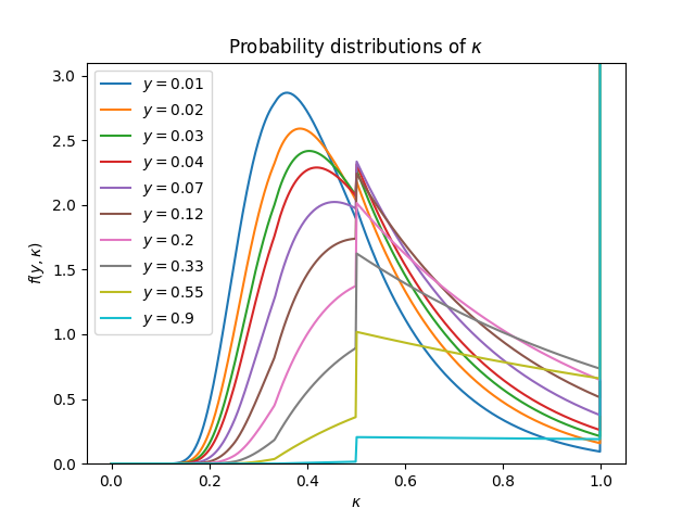
Plots of the probability density functions

Here are plots of the function $f(y,\kappa)$ whose expression is given by Equation 30:

infinite

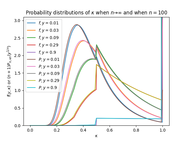
We can compare it with a plot of the distributions when $n$ is finite (say, $100$), and we may see that they are very close:

infinite 2

We have not investigated the asymptotic behavior of the error if we approximate the distribution with finite $n$ by the distribution with infinite $n$, but we may expect that the error is small enough for applicational uses when $n$ is a usual note count in a rhythm game chart (usually at least $500$).

Moments

It may be interesting to calculate the moments of the distribution.

We need to evaluate

$$\mu_\nu\!\left(y\right)\coloneqq\int_0^1\kappa^\nu f\!\left(y,\kappa\right)\mathrm d\kappa.$$

First, calculate

$$\begin{align*} &\phantom{=~}\int_0^{\frac1s}\kappa^\nu\left(\ln y^{s\kappa-1}\right)^jy^{s\kappa-1}\ln y\,\mathrm d\kappa\\ &=\int_{y^{-1}}^1\left(\frac{\log_yw+1}{s}\right)^\nu\left(\ln w\right)^j\,\mathrm dw\\ &=\frac1{s^{\nu+1}}\sum_{p=0}^\nu\binom\nu p\frac1{\left(\ln y\right)^p} \int_{y^{-1}}^1\left(\ln w\right)^{j+p}\,\mathrm dw\\ &=\frac{1}{s^{\nu+1}}\sum_{p=0}^\nu\binom\nu p\frac{\left(-1\right)^{j+p}\left(j+p\right)!}{\left(\ln y\right)^p} \left(1-y^{-1}\sum_{l=0}^{j+p}\frac{\left(\ln y\right)^l}{l!}\right). \end{align*}$$

$$\begin{align*} &\phantom{=~}\int_0^{\frac1s}\kappa^\nu\Delta g_s\!\left(y,\kappa\right)\mathrm d\kappa\\ &=\sum_{j=0}^s\left(-1\right)^s\frac{A_{s,j}}{j!} \frac{1}{s^{\nu+1}}\sum_{p=0}^\nu\binom\nu p\frac{\left(-1\right)^{j+p}\left(j+p\right)!}{\left(\ln y\right)^p} \left(1-y^{-1}\sum_{l=0}^{j+p}\frac{\left(\ln y\right)^l}{l!}\right)\\ &=\frac{\left(-1\right)^s}{s^{\nu+1}}\sum_{p=0}^\nu\binom\nu p\frac{\left(-1\right)^p}{\left(\ln y\right)^p} \left( \sum_{j=0}^s\frac{\left(j+p\right)!\left(-1\right)^j}{j!}A_{s,j} \right.\\&\qquad\qquad\qquad\qquad\qquad\qquad\left.{} -y^{-1}\sum_{j=0}^s\frac{\left(j+p\right)!\left(-1\right)^j}{j!}A_{s,j}\sum_{l=0}^{j+p}\frac{\left(\ln y\right)^l}{l!} \right). \end{align*}$$

Define

$$B_{s,l,p}\coloneqq\sum_{j=\max(0,l-p)}^s\frac{\left(j+p\right)!\left(-1\right)^j}{j!}A_{s,j},$$

$$(31)$$

$$D_{\nu,p,l}\coloneqq\sum_{s=\max(1,l-p)}^\infty\frac{\left(-1\right)^s}{s^{\nu+1}}B_{s,l,p}.$$

$$(32)$$

Then,

$$\begin{align*} &\phantom{=~}\int_0^{\frac1s}\kappa^\nu\Delta g_s\!\left(y,\kappa\right)\mathrm d\kappa\\ &=\frac{\left(-1\right)^s}{s^{\nu+1}}\sum_{p=0}^\nu\binom\nu p\frac{\left(-1\right)^p}{\left(\ln y\right)^p} \left(B_{s,0,p}-y^{-1}\sum_{l=0}^{s+p}B_{s,l,p}\frac{\left(\ln y\right)^l}{l!}\right). \end{align*}$$

$$\begin{align*} &\phantom{=~}\int_0^1\kappa^\nu g\!\left(y,\kappa\right)\mathrm d\kappa\\ &=\sum_{s=1}^\infty \frac{\left(-1\right)^s}{s^{\nu+1}}\sum_{p=0}^\nu\binom\nu p\frac{\left(-1\right)^p}{\left(\ln y\right)^p} \left(B_{s,0,p}-y^{-1}\sum_{l=0}^{s+p}B_{s,l,p}\frac{\left(\ln y\right)^l}{l!}\right)\\ &=\sum_{p=0}^\nu\binom\nu p\frac{\left(-1\right)^p}{\left(\ln y\right)^p} \left(D_{\nu,p,0}-y^{-1}\sum_{l=0}^\infty D_{\nu,p,l}\frac{\left(\ln y\right)^l}{l!}\right). \end{align*}$$

Now, the only problem is how to get $D_{\nu,p,l}$. Substitute Equation 26 into Equation 31, and after some calculations, we can get the general formula of $B_{s,l,p}$:

$$B_{s,l,p}=\frac{\left(-1\right)^s\max(l,s+p-2)!}{\left(s-1\right)!}\cdot\begin{cases} p\left(p-1\right),&l\in0\,..s+p-2,\\ p-s,&l=s+p-1,\\ 1,&l=s+p. \end{cases}$$

Substitute it into Equation 32, and notice the edge cases, we can get

$$\begin{align*} D_{\nu,p,l}&=\begin{cases} p\left(p-1\right)\sum_{s=1}^\infty\frac{\left(s+p-2\right)!}{s^{\nu+1}\left(s-1\right)!}, &l\in0\,..p-1,\\ p!\left(p-1\right)+p\left(p-1\right) \sum_{s=2}^\infty\frac{\left(s+p-2\right)!}{s^{\nu+1}\left(s-1\right)!}, &l=p,\\ \begin{split} &\textstyle{\frac{l!}{\left(l-p\right)^{\nu+1}\left(l-p-1\right)!} -\frac{l!\left(2p-l-1\right)}{\left(l-p+1\right)^{\nu+1}\left(l-p\right)!}}\\ &\qquad\textstyle{ {}+p\left(p-1\right)\sum_{s=l-p+2}^\infty\frac{\left(s+p-2\right)!}{s^{\nu+1}\left(s-1\right)!},} \end{split} &l\in p+1\ldots\infty \end{cases}\\ &=\begin{cases} p\left(p-1\right)\left(\left(p-1\right)!+S_{\nu,p}\right),& l\in0\,..p,\\ \begin{split} &\textstyle{\frac{l!}{\left(l-p\right)^{\nu+1}\left(l-p-1\right)!} -\frac{l!\left(2p-l-1\right)}{\left(l-p+1\right)^{\nu+1}\left(l-p\right)!}}\\ &\qquad\textstyle{ {}+p\left(p-1\right)\left(S_{\nu,p}-\sum_{s=2}^{l-p+2}\frac{\left(s+p-2\right)!}{s^{\nu+1}\left(s-1\right)!}\right),} \end{split} &l\in p+1\ldots\infty, \end{cases} \end{align*}$$

where the infinite sum

$$S_{\nu,p}\coloneqq\sum_{s=2}^\infty\frac{\left(s+p-2\right)!}{s^{\nu+1}\left(s-1\right)!}.$$

There is no closed form for $S_{\nu,p}$, but we may express it in terms of Stirling numbers of the first kind and the Riemann $\zeta$ function. For $p\in1\,..\nu$, we have

$$\begin{align*} S_{\nu,p}&=-\left(p-1\right)!+\sum_{s=1}^\infty\frac{s\left(s+1\right)\cdots\left(s+p-2\right)}{s^{\nu+1}}\\ &=-\left(p-1\right)!+\sum_{s=1}^\infty\frac1{s^{\nu+1}}\sum_{\lambda=0}^{p-1}\begin{bmatrix}p-1\\\lambda\end{bmatrix}s^\lambda\\ &=-\left(p-1\right)!+\sum_{\lambda=0}^{p-1}\begin{bmatrix}p-1\\\lambda\end{bmatrix}\zeta\!\left(\nu-\lambda+1\right), \end{align*}$$

where $\begin{bmatrix}\cdot\\\cdot\end{bmatrix}$ denotes (unsigned) Stirling numbers of the first kind. For $p=0$, we have

$$\begin{align*} S_{\nu,0} &=\sum_{s=2}^\infty\frac1{s^{\nu+1}\left(s-1\right)}\\ &=\sum_{s=2}^\infty\frac1{s^{\nu+1}\left(s-1\right)}-\sum_{s=2}^\infty\frac1{s\left(s-1\right)}+1\\ &=1-\sum_{s=2}^\infty\frac1{s^{\nu+1}}\frac{s^\nu-1}{s-1}\\ &=\nu+1-\sum_{s=1}^\infty\frac1{s^{\nu+1}}\sum_{\lambda=0}^{\nu-1}s^\lambda\\ &=\nu+1-\sum_{\lambda=0}^{\nu-1}\zeta\!\left(\nu-\lambda+1\right). \end{align*}$$

Then, the following steps will be extremely tedious, and I doubt there will be a closed form for our final result, so I will not continue to find the general formula for the moments.

---

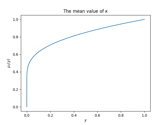
However, we may obtain the first moment (mean) analytically. We have

$$D_{1,0,l}=\begin{cases}-1,&l=0,\\\frac1l-\frac1{l+1},&l\in1\ldots\infty,\end{cases} \quad D_{1,1,l}=\begin{cases}0,&l=0,1,\\\frac1l+\frac1{l-1},&l\in2\ldots\infty.\end{cases}$$

$$\begin{align*} \mu_1\!\left(y\right) &\coloneqq\int_0^1\kappa f\!\left(y,\kappa\right)\mathrm d\kappa\\ &=y+y\int_0^1\kappa g\!\left(y,\kappa\right)\mathrm d\kappa\\ &=\frac{\operatorname{li}y-\ln(-\ln y)-\gamma}{\ln y}, \end{align*}$$

where $\operatorname{li}$ is the logarithmic integral function, and $\gamma$ is the Euler–Mascheroni constant. The function seems undefined when $y=0$ or $y=1$, but it has limits at these points:

$$\mu_1\!\left(y\to0^+\right)=0,\quad\mu_1\!\left(y\to1^-\right)=1,$$

which is intuitive. (This function tends to $0$ very slowly when $y\to0^+$, so slowly that I almost did not believe that when I did the numerical calculation first.)

The plot:

mean

We should also be able to find other statistical quantities like the median, the mode, the variance, etc., but they seem do not have closed forms.

Some interesting observations

The probability distribution of $\kappa$ seems to tend to be a uniform distribution plus a Dirac $\delta$ distribution when $y$ is very close to $1$. This phenomenon is very visible if we look at the plot of $f(y=0.9,\kappa)$.

In other words, the distribution seems like

$$f(y\approx1,\kappa)\approx \left(1-y\right)U\!\left(\frac12,1\right)+y\delta(\kappa-1),$$

where $U(a,b)$ denotes the uniform distribution on the interval $[a,b]$.

This can be justified by expanding $f(y,\kappa)$ in Taylor series of $1-y$ and retaining the first-order terms only. Note that

$$y^a\left(\ln y\right)^b= \left(y-1\right)^b\left(1+\left(\frac b2-a\right)\left(1-y\right)+\cdots\right),$$

so the only case where the Taylor series has a non-zero first-order term is when $b=1$ or $b=0$. In Equation 30, we can see that the power on $\ln y$ is at least one for each term (because of the general $\ln y$ factor in front), so only the terms with no $\ln y$ factors but the general one will have a first-order term. In this case, the first order term is proportional to $y-1$, and the proportional coefficient is just the coefficient in the front of the term in $f$, which is independent of $\kappa$ because $\kappa$ only appears in the power index of $y$.

Therefore, we may see that only $q=1$ and $q=2$ terms have a non-zero first-order term, and they are respectivey $-2\left(y-1\right)$ and $2\left(y-1\right)$. This means that when $y$ is very close to $1$,

$$f(y\approx 1,\kappa)\approx\begin{cases} 2\left(1-y\right),&\kappa\in\left(\frac12,1\right),\\ 0,&\kappa\in\left(0,\frac12\right). \end{cases}$$

This is exactly the uniform distribution.

There is an intuitive way to explain the appearance of the uniform distribution. When $y$ is very close to $1$, the probability of getting one combo break ($1-Y$) is already very small, so it is very unlikely that there are two or more combo breaks. Assuming there is only one combo break and it may appear anywhere with equal probability. The combo break will cut the string of notes into two pieces, and the length of the larger piece is the max combo, which is uniformly distributed between half note count and full note count.

---

Every rhythm game player knows: never celebrate too early. You never know whether you will miss near the end. It is then interesting to know what is the probability of getting almost a full combo, i.e. what is the probability of getting $\kappa$ very close to $1$.

If we find the limit of $f(y,\kappa)$ as $\kappa\to1^-$, it is

$$f\!\left(y,\kappa\to1^-\right)=-2y\ln y.$$

There is a peak of this probability density at $y=\mathrm e^{-1}$. Therefore, when $y=\mathrm e^{-1}$, the probability of getting $\kappa$ very close to $1$ is the largest.

When does $y=\mathrm e^{-1}$, then? Because

$$y=Y^n=\left(1-\frac{n_\mathrm b}n\right)^n,$$

where $n_\mathrm b$ is the average number of combo breaks, then it tends to $\mathrm e^{-n_\mathrm b}$ when $n\to\infty$. Therefore, the probability of getting almost a full combo is the highest when your average number of combo breaks is exactly one.

---

From the plot, it seems that the probability of getting $\kappa$ a little bit higher than $\frac12$ is always higher than the probability of getting $\kappa$ a little bit lower than $\frac12$. According to Equation 28, the jump in $f(y,\kappa)$ at $\kappa=\frac12$ is

$$f\!\left(y,\kappa\to\frac12^+\right)-f\!\left(y,\kappa\to\frac12^-\right)=-2y\ln y.$$

Interestingly, this coincides with $f\!\left(y,\kappa\to1^-\right)$.

---

Define

$$y_0(\kappa)\coloneqq\mathop{\mathrm{arg\,max}}_{y\in[0,1]}\,f(y,\kappa),$$

and then it seems that $y_0:[0,1]\to[0,1]$ is injective but not surjective. It is strictly increasing, and there is a jump at $\kappa=\frac12$ and at $\kappa=1$.

It has an elementary expression on $\left[\frac12,1\right)$:

$$y_0\!\left(\kappa\in\left[\frac12,1\right)\right) =\exp\frac{-2\kappa+1+\sqrt{2\kappa^2-2\kappa+1}}{\kappa\left(\kappa-1\right)}.$$

Some applications

In Phigros, one should combo at least $60\%$ of the notes to get a white V () rank. If on average I have one combo break in a chart, which has $1300$ notes, what is the probability of comboing at least $60\%$ of the notes in the chart?

Solution. The success rate is

$$Y=\frac{1300-1}{1300},\quad y=Y^{1300}\approx\mathrm e^{-1}.$$

The probability of comboing more than $60\\%$ of the notes is

$$\begin{align*} &\phantom{=~}\int_{60\%}^1f\!\left(y,\kappa\right)\mathrm d\kappa\\ &=y+\int_{0.6}^1-y^\kappa\ln y\left(2+\ln y^{\kappa-1}\right)\mathrm d\kappa\\ &\approx\mathrm e^{-1}+\int_{0.6}^1\mathrm e^{-\kappa}\left(3-\kappa\right)\mathrm d\kappa\\ &=\frac75\mathrm e^{-\frac35}\\ &\approx0.768. \end{align*}$$

---

Oh, my god! It is hard to come up with application problems. I hope readers find out the applications themselves.