Jekyll2026-04-30T17:49:58-07:00https://ulysseszh.github.io/feed/tags/ode.xml<![CDATA[Ulysses’ trip]]>Here we are at the awesome (awful) blog written by UlyssesZhan!UlyssesZhanulysseszhan@gmail.com<![CDATA[From Picard iteration to Feynman path integral]]>2025-11-13T17:31:24-08:002025-11-13T17:31:24-08:00https://ulysseszh.github.io/physics/2025/11/13/picard-path-integralDiscrete path integral
As we all know, the Schrödinger equation is where is the state vector and is the Hamiltonian operator (may be time-dependent). This is an ordinary differential equation (ODE), so we can express its solution as a sum where each term in the sum is defined iteratively by (see also my past article) This iteration is called the Picard iteration, which is most known as a method to prove the Picard–Lindelöf theorem.
Let us actually write out the general term in this sum as where
Now with the trick of time-ordering, we can rewrite this as
where means to order the operators inside according to their time arguments. The factor of appears because there are ways to order time variables, but another way to see this is to note that the domain of integration is an -simplex, whose volume is of the corresponding -parallelotope. When we then sum over all , we get the time-ordered exponential The operator has a bunch of equivalent names, such as the time evolution operator, the propagator, the Green’s function, the Dyson operator, and the S-matrix (well, they are not entirely equivalent because they are used under different contexts).
The interesting part comes when we consider the matrix elements of and how they relate to the matrix elements of . We choose an orthonormal basis , and then insert a between each pair of Hamiltonian operators in the expression of :
where we have abbreviated , and are a specific ordering of the integrated time variables. We can pull out the sum over intermediate basis states and call the summand a contribution from a walk 1 from to . In other words, where the sum is over all walks of length from to , and Now, the matrix elements of the full propagator is then the sum over contributions from all walks:
We can imagine a “Hamiltonian graph” formed by taking the basis states as vertices and the Hamiltonian matrix elements as edge weights (the weight of the directed edge from to is ). Note that an edge can be a self-loop. Then, the propagator contribution from a walk is given by integrating the product of all the edge weights along the walk (for a trivial walk, which has zero length, the contribution is simply ). This formulation may be called the discrete path integral. There is a paper on arXiv that delivers the idea of the Hamiltonian graph. Its difference from the current article is that it only focuses on time-independent Hamiltonians and that it treats self-loops separately instead of just like normal edges. The following two sections (excluding self-loops and the Feynman path integral) largely follow from the ideas from this paper.
Excluding self-loops
In some cases, it may be hard to consider self-loops on the Hamiltonian graph. We may then benefit from counting only walks without self-loops. However, the contributions from each walk will now be different because we have to account for the same walk with self-loops inserted at various positions. In other words, for a walk without self-loops, instead of contributing , we now want to find the contribution that sums over all ways to insert self-loops into : where is the number of self-loops inserted at the vertex , and is an abbreviation of this walk:
I will show that we can find an expression for for the case when the Hamiltonians at different times commute with each other. In this case, we have Therefore, by the definition of , we have
For abbreviation, for the rest of this section, we denote .
Now, we use a trick to replace the factorial in the denominator with an contour integral: where the contour is a counterclockwise simple closed curve around the origin in the complex plane. We then have
We have thus separated the sums over different . Each sum is a geometric series that converges when we choose the contour large enough, so
where the last step used the residue theorem for each pole at . This expression is exactly the expanded form of the divided difference of , often denoted . Therefore,
The discrete path integral can then be rewritten in a form that only involves collecting contributions from walks without self-loops:
Feynman path integral
This discrete path integral formulation of the propagator already looks similar to the Feynman path integral, but we have to go a step further to take the continuum limit to actually get there. For simplicity, I will only consider a particle with unvarying mass moving in a time-independent potential in one dimension. Its Hamiltonian is , and the orthonormal basis is chosen to be the position basis, also denoted as .
The more standard way to derive the Feynman path integral is to slice the time integral in Equation 1, to express the total exponentiation as a product as many small exponentiations, and then to insert between each pair of exponentiations (see, e.g., chapter 6 of Quantum Field Theory by Mark Srednicki). However, this approach does not make its connection to the discrete path integral clear. Instead, we will discretize the position space into a lattice with spacing , use the discrete path integral formulation on this lattice, and then take the continuum limit at the end. Now, instead of , we have . Each basis vector now has two nearest neighbors and .
In the position basis, the kinetic part of the Hamiltonian is a second derivative operator. From numerical differentiation, we can approximate it on the lattice as Therefore, the discretized Hamiltonian is
Its matrix elements are then
Conceptually, it consists of on-site energy and nearest-neighbor hops. The on-site energy looks bothersome, but we can remove it if we only consider walks without self-loops. Equation 2 becomes where is the imaginary time, and is defined for the same abbreviation reason as the previous section. The terms proportional to in the multiplicant are omitted because we only consider walks without self-loops. The rest of this section is done under a Wick rotation so that is assumed to be a positive real parameter.
First, let us tackle the divided difference . Define , where is the mean of . Then,
is of order unity (while is of order , which is much larger than unity for small ). Then, from the expanded form of the divided difference, we can easily get Recalling how we initially derived the divided difference, we have
When
is large (the reason of which will be explained in a minute), we have etc., while is of the order of unity, so we only need to consider the terms with the lowest . The leading term is the term with , which is trivially , so we have This contributes to the potential part of the action.
Substitute Equation 4 into Equation 3, and we have
where is a large positive number when is small. Observe that the factor is the probability mass function of the Poisson distribution with mean evaluated at . When is very large, the Poisson distribution can be approximated by a delta distribution because the standard deviation is much smaller than . In other words, . Therefore,
Imaginary parameter Poisson distribution
It was this point that got me thinking the most when I originally tried to derive the Feynman path integral without the Wick rotation. While the approximation is valid, the problem is whether we can likewise say (or ). While it is true that the left-hand side has a very large magnitude when so that it dominates the sum, it does not actually approximate the right-hand side because the right-hand side is of order unity and is real. In fact, the summand is rapidly oscillating when is near , so the numbers of different phases actually cancel each other out and give a number with small magnitude in the end.
If you actually try to walk through the calculation without the Wick rotation, you will find that what you need to justify in the end is something like this (there are some other factors dependent on in the summand, but we can remove them by some techniques, so let us ignore them for simplicity): where and are both large positive numbers. This is unfortunately false, neither in magnitude nor in phase, and not even up to an overall factor.
While it is true that a lot of things can be carried over by analytic continuation, which is the reason why the Wick rotation can give the correct result in many cases, you can do the analytic continuation only if every step you take is actually analytic. Having an approximation based on the magnitude of each summand is not analytic because a fast oscillation can change the result drastically. Therefore, I am not satisfied with this derivation with the Wick rotation, but I have not found a better way to do it yet.
If the factor involving were not there in the summand, the sum of products is exactly the probability that a random walk starting at ends at after steps, where at each step the walk moves to the left or right nearest neighbor with equal probability . Instead of considering one random walk with steps, we can consider random walks with steps each, where both and are large. Because is large, we can approximate the distribution of the position at the end of the th random walk as a normally distributed random variable with variance . Note that even though is large, is still very small, so the majority of contribution in the sum only comes from those paths where
does not differ too much from the of its corresponding part of random walk. Therefore, if we fix a set of , the factor involving in the summand can be approximated by replacing with for all in the th random walk segment. We can then pull this factor out of the sum over (but still inside the integral over
). Therefore, we get where the extra factor of in the multiplicant comes from converting a probability density to a probability (since the probability that the position ends up at the lattice site is times the probability density at ).
Combining the product of exponentiations into the exponentiation of a sum, we have If we introduce the time step , for large , we have
Similarly, for the potential part we introduce the time step 2, Here, and
are the position and its time at time for a particle undergoing these random walks. Therefore, we have
Finally, simply revert the Wick rotation by substituting and rewrite the integral over as a path integral over all paths . Then, we get the Feynman path integral expression of the propagator: This completes the derivation.
You may wonder why I use the word “walk” while the resultant thing is called a “path” integral. This is just because “walk” is the correct term in graph theory that describes the object we use here, and the sum over all the walks is called a “path” integral because it is what physicists call. In graph theory, however, a path is a walk in which all vertices are distinct.↩︎
]]>UlyssesZhanulysseszhan@gmail.com<![CDATA[Eigenfunctions of the Laplacian on an annulus with homogeneous Neumann boundary condition]]>2025-04-11T00:40:49-07:002025-04-11T00:40:49-07:00https://ulysseszh.github.io/math/2025/04/11/laplacian-annulusThe problem and the solution
Suppose there is an annulus defined by the region . What are the functions defined on this region that satisfy
and the boundary conditions
i.e., eigenfunctions of the Laplacian on the annulus with homogeneous Neumann boundary conditions?
For any boundary condition with azimuthal symmetry, an easy separation of variable gives you solutions of the general form where ,
, and are constants fixed by the boundary conditions, and is an integer and the azimuthal quantum number. The functions and are Bessel functions of the first and second kind, respectively, which are two linearly independent solutions of the Bessel equation with some particular normalization. Plugging the general form into the boundary condition, and we have where
. This is regarded as a homogeneous linear system of equations for and . In order for it to have nontrivial solutions, the determinant of the coefficient matrix must vanish, which gives We can then assign a radial quantum number to the eigenfunctions by making the value of the th root of , which we may casually call
.
We then have the final solution (up to normalization)
where is the azimuthal quantum number, and is the radial quantum number, and is defined as the th root of the function . The eigenvalue is . In order for the eigenfunctions to be complete, we need to allow to be any integer, but we will restrict ourselves to non-negative in the rest of the article because the negative ones are practically the same as the positive ones.
Distribution of eigenvalues
From the well-known asymptotic form of the Bessel functions (source) we can easily conclude that the asymptotic form of is This inspires us to define a function in companion with as which will have the asymptotic form Therefore, and are like the cosine and sine pair of oscillatory functions, with a phase angle asymptotically directly proportional to .
Here is a plot that shows how behaves:
The blue line is , and the orange line is . we can see that the two functions are asymptotically equal.
A good thing about this description is that we can now see that as a root of is just the solution to the equation . In other words, are just the points at which the blue line crosses the horizontal axis in the plot above. Therefore, if we can find the inverse function (maybe in a series expansion), we can directly get . We can see from the plot that is probably not a good enough approximation. Therefore, we would like to seek higher order terms.
Kummer’s equation
For this part, we employ a method similar to a paper by Bremer.
First, for a general homogeneous second-order linear ODE in the form , where and are known functions of , we can define and the ODE will become a normal form . Therefore, for any second-order linear ODE, we only need to consider those without the first-derivative term.
Then, one can prove that, for the ODE , its two linearly independent solutions can be expressed as where satisfy Kummer’s equation This may seem like converting a problem to a more complicated one, but the advantage is that is not oscillatory while and are oscillatory, which means that it would be easier to expand
as a series for large . Notice that , which provides a means of finding if the solutions of the original ODE are known.
Derivation
For the ODE , substitute the trial solution , where are real functions of . We can derive the following equations: The first equation gives , which we can substitute into the second equation to get Equation 5. On the other hand, the real and imaginary parts of the trial solution gives us Equation 4. Technically speaking, it can be called the real and imaginary parts only if , but they are still solutions to the ODE.
Another way to prove Kummer’s equation is just substituting and check that it satisfies Kummer’s equation if and satisfy the ODE and have Wronkskian equal to .
Now, we can try to apply this to and . First, we need to find the second-order ODE that those two functions satisfy. We already know that and are solutions to Equation 1, so it would be straightforward to derive that and satisfy
To reduce this into the normal form without the first-derivative term, define and we have
and satisfy . Equation 4 then gives (the normalization of and the initial value of are chosen to make sure they are correct). You may worry that is imaginary, but will be negative in that region so that everything works out and is real in the end. Substitute Equation 7 into Equation 3 and 2, and we have where . By this, we have a workable expression for so that we now just need to turn our attention to .
We can substitute in Equation 6 into Equation 5 and expand on both sides as a series of at infinity and solve for the series coefficients to get which has a certain convergence radius which is not important at this stage.
Asymptotic expansion
Here we will work out another way of expanding as a series based on properties of the Bessel functions. From Equation 7, we have If we were working with
instead, we would be able to employ the handy Nicholson’s integral, but the same method cannot be applied here.
Why it does not work
Nicholson’s integral is where is the modified Bessel function. A derivation is given in Section 13.73 of Watson’s A Treatise on the Theory of Bessel Functions.
To apply this to , we need to use (source) Then, we just need to work out the cross terms
. By the same method of deriving Nicholson’s integral, we can get
which is a more general version of Nicholson’s integral. However, this formula is only valid for because otherwise the integral diverges near , while we need .
One can also try to employ the same method of deriving Nicholson’s integral directly on , but it will turn out to have the same divergence problem. Briefly speaking, there is a term that is an infinitesimal quantity times the integral of , which can only be thrown away without any problem if , which is not the case here.
We can, however, use the asymptotic expansion of the Bessel functions directly (source):
where where the raising factorial notation is used. By combining them, we get
Derivation
First, expand the squares, and the cross terms will cancel, and we have
For the first term, combine a and a to get a , so that we can resum it as
Similarly, for the other term, combine a and a to get a , so that we can resum it as
Combine to get
Then, take the reciprocal of the series, and we have where
is defined recursively as (noticing that )
Series reciprocation
For a series , what is the reciprocal ? Assume that it is another series . Then, we have
Compare the coefficients of
on both sides, and we have Therefore, we get the recursion relation I will use the notation of superscript for series reciprocation in the rest of this article.
There are non-recursive ways of writing those coefficients, but they are either very long or needs notations that require a bit of explanation, so I restrained from that.
Therefore, we get the asymptotic expansion of as
(with understood as ; I will be assuming the reference to any expansion coefficients outside their designated range to be interpreted as zero in all occurrences in the rest of this article). The additive constant in is properly chosen so that Equation 7 is satisfied without being off by a phase (but it is actually unimportant anyway because it gets canceled in the expression of ). One can check that this agrees with Equation 8.
We can now find an expansion for :
Then it is the final step to find an expansion for the inverse function . Take the reciprocal of :
Then, invert the series:
where is the Bell polynomial. Finally, take the reciprocal:
The first few terms are (I only write two terms here because the next term starts to be very long; it will turn out that only the first two terms are useful anyway).
(The capitalized R is the parameter in this article; I have so poor choices of variable names…)
The result is shown in the plot below.
The black line is the exact function for , , and the blue, green, orange, and red lines are the truncated asymptotic series of the inverse function with 1, 2, 3, and 4 terms, respectively. The horizontal grid lines are the integer multiples of , whose intersections with the black line gives the wanted roots . To be honest, the result is a bit anticlimactic because it turns out that truncating the series to only the first two terms gives the best approximation. This is within expectation, though, because the asymptotic series is never guaranteed to give better approximations with more terms.
The mode
For all the previous plots, I have only shown . For being other positive integers, they all look similar, but there is a special feature for . To see this, first study the limiting form of and for small . The limiting forms of the Bessel functions are (source) We can then get
From this, we can get the limiting form of : The particularly interesting thing to note is the negative sign for the case of
. Remember that , which is a positive thing, we would conclude that would become zero for some positive if , while that may not be the case for . Indeed, there is no positive for if , as we can see from the plot below.
The red line is for , which we can see that crosses the horizontal axis, while the blue line is for , which does not cross the horizontal axis. The more lightly colored lines are the limiting forms of for small .
The implication is that the mode would not exist for but exist for . However, traditionally, when people talk about eigenmodes of the Laplacian, the quantum number refers to the 1-based numbering of the roots of the Bessel functions ( in our case). This would mean that what is referred to as the mode in this article would be traditionally called the mode, while the mode in this article is the same as what is traditionally called. In other words, the traditional names of the modes for different values of are
Another way to see this is that, according to Equation 7, in order for and to be real-valued, whenever , we would need to be purely imaginary, and vice versa. From Equation 6, we can see that is real when , and it is purely imaginary when . Therefore, goes from negative to positive when
crosses . This means that is monotonically decreasing when but monotonically increasing when , and is the minimum. This means that which means . This means that when , the root
must exist, and we also get a lower bound . However, when , would be monotonically increasing for all , and thus would be positive for all , which means that does not exist. By a similar method, we can also derive an upper bound for . We have
which means . This means that . This also implies the nonexistence of .
Maybe we can still formally define , and the eigenfunction would be the trivial with a zero eigenvalue.
Numerical root-finding
A key thing to note about the asymptotic series truncated to the first two terms is that it is impossible to get values smaller than a certain bound: where the equality holds when . This means that if we use to approximate the roots, we will miss all the roots with . The number of missed roots is (this includes the mode, so for , the number of missed roots is ). According to the bound on we derived in the previous section, all the missing roots are in the interval
. In order to numerically find those roots, we can equispacedly sample more than points (maybe points to be safe) in the interval as initial guesses and use usual root-finding methods such as Newton’s method to find the roots.
Limiting cases
The disk limit
When , the annulus becomes a disk. We will see how the eigenmodes tend to the eigenmodes on a disk, which are given by where are the roots of .
In this case, we can regard as small, so using Equation 9 gives
This means that or just . We can also see this by noting that
when , so . Therefore, the solutions to would just be the solutions to , which are just roots of . This hence recovers the eigenmodes on a disk.
The circle limit
When , the annulus becomes a circle. In this case, we can suppress the radial dimension to make the problem one-dimensional. The eigenmodes would be and the eigenvalues are (no need to distinguish between and here).
This case is interesting in that the radial dimension would become “invisible” from the physics of the system. Note that would be a very flat line, which means that would need to increase by a very large amount in order to get to increase by . Therefore, the radial quantum number would be very hard to increase. Formally, the eigenvalues of the modes with will become infinite, so we then practically only need to consider for the “low-energy description” of the system.
We have previously derived the lower bound and upper bound for , which gives . When , we then get by the squeeze theorem. The eigenvalue of the Laplacian is then
.
For the case of , there are two ways to look at it. If we do not regard the trivial mode as a mode, then we can say that the mode does not exist on a circle, which fits nicely with the fact that the mode does not exist for in the annulus. With the other way, if we regard the and mode on the annulus as the trivial mode , then it also nicely tends to the trivial mode on the circle in the limit .
The homogeneous Dirichlet boundary condition
So far I only talked about the homogeneous Neumann boundary condition. In the case of homogeneous Dirichlet boundary condition most of the derivation is the same, but with
There is a qualitative difference from the Neumann case, though, which comes from the limiting behavior of : We can see that they are positive in both cases, which means that
does not have a positive solution in both cases. Therefore, the radial modes start at for all (in contrast to the Neumann case where mode exists for ). The traditional naming of the eigenmodes then agrees with .
An implication of the difference is that there is no longer a non-trivial circle limit. This is because the eigenvalue of any mode with positive would tend to infinity as .
]]>UlyssesZhanulysseszhan@gmail.com. The limiting cases of a disk and a circle are discussed.]]><![CDATA[Solving ODE by recursive integration]]>2022-11-15T15:02:30-08:002022-11-15T15:02:30-08:00https://ulysseszh.github.io/math/2022/11/15/ode-recursiveThe method
Suppose we have an ODE (with initial conditions) where is the unknown function, and is Lipschitz continuous in its first argument and continuous in its second argument. By Picard–Lindelöf theorem, we can seek the unique solution within .
Here, I propose the following method: we can write out a sequence of functions defined by (the properties of guarantee that the integral is well-defined). Then, if the sequence
converges uniformly on (question: can this condition actually be proved?), then the sequence converges uniformly to a function on , which is the unique solution to Equation 1.
Proof
The proof is easy. Note from Equation 3 that Then, take the limit . By the uniform convergence, we recovers Equation 1.
An example
Suppose and , then This is because
By taking the limit , we get
, which means that the unique solution to with initial condition is , expectedly.
Approximation
This method is good because integration is sometimes much easier than solving ODE. We can use integration to get functions that are close to the exact solution. A natural question to ask is how close is to the exact solution .
If Equation 1 is defined on (where we may define differences and infinitesimals), it is clear that is an infinitesimal of higher order than .
]]>UlyssesZhanulysseszhan@gmail.com from , we can get the solution of the ODE
with initial conditions as the limit of the sequence of functions.]]><![CDATA[Solving linear homogeneous ODE with constant coefficients]]>2022-11-06T16:42:48-08:002022-11-06T16:42:48-08:00https://ulysseszh.github.io/math/2022/11/06/linear-ode-solutionThis article is translated from a Chinese article on my Zhihu account. The original article was posted at 2019-04-06 13:46 +0800.
Notice: Because this article was written very early, there are many mistakes and inappropriate notations.
(I’m going to challenge writing articles without sum symbols!)
In this article, functions all refer to unary functions; both independent and dependent variables are scalars; and differentials refer to ordinary differentials.
Definition 1 (linear differential operator). Let be a differential operator. If for any two functions and constants , the operator satisfies
then is a linear differential operator.
Lemma 1. The sufficient and necessary condition for to be a linear differential operator is that for any tuple of functions and any tuple of constants (the dimensions of the two vectors are the same), the operator satisfies
Brief proof. Directly letting and be 2-dimensional vectors and using Definition 1, the sufficiency can be proved; by using mathematical induction on the dimension of and , the necessity can be proved.
Definition 2..
Lemma 2. Suppose the -dimensional vector is independent to , and is a sequence of functions, then
Brief proof. By mathematical induction.
Lemma 3. Suppose is a tuple of functions w.r.t. , and the dimension of is , then the differential operator is a linear differential operator.
Brief proof. By Definition 1.
Corollary of Lemma 3. Suppose is a constant -dimensional vector, then the differential operator is a linear differential operator.
Lemma 4 (associativity).
Proof is omitted.
Definition 3 (linear differential operator with constant coefficients). Linear differential operators with form as Equation 1 are called linear differential operators with constant coefficients.
Definition 4 (linear ODE). Suppose is a linear differential operator. Then the ODE w.r.t. the function is called a linear ODE, where is a function.
Specially, if , the ODE is called a homogeneous linear ODE. If is a linear differential operator with constant coefficients, then the ODE is called a linear ODE with constant coefficients.
Definition 5 (generating function). For a sequence , the function is called the (ordinary) generating function (OGF) of the sequence.
Note. here we do not introduce vectors with infinite dimensions. Actually,
Definition 6 (exponential generating function). For a sequence , the OGF of the sequence is called the exponential generating function (EGF) of the sequence . In other words,
Lemma 5 (differential of power functions). Suppose , then
Note. it is stipulated that factorials of negative integers are infinity, so when .
Brief proof. By mathematical induction.
Lemma 6 (differential of EGF). If is the EGF of a sequence , then is the EGF of .
Proof. Then the result can be proved by Definition 6.
Corollary to Lemma 6.
Lemma 7 (associativity).
Proof is omitted.
Definition 7 (zero function). The function whose value is always zero whatever the value of the independent variable is is called the zero function.
Lemma 8. The sufficient and necessary condition for the OGF/EGF of a sequence to be zero function is that for any .
Brief proof. The sufficiency can be proved by Definition 6 and Definition 7; the necessity can be proved by Taylor expansion of the zero function.
Definition 8.
Lemma 9 (distributivity).
Proof is omitted.
Definition 9 (sequence equation). Let be an unknown sequence. If the function explicitly depends on terms in the sequence, then the function is called a sequence equation w.r.t. the sequence . For a sequence, if it satisfies the equation for any , then it is called a special solution of the sequence equation. The set of all special solutions of the sequence equation is called the general solution of the equation.
Definition 10 (linear dependence of sequences). If for a set of sequences (a sequence of tuples) there exists a tuple of constants which are not all zero (the dimensions of and are the same) such that for any , then the set of sequences are called to be linearly dependent. They are otherwise called to be linearly independent.
Lemma 10. The sufficient and necessary condition for a set of sequences to be linearly dependent is that
Proof. First prove the necessity. There exists a tuple of constants which are not all zero such that for any (Definition 10).
Replace by respectively, and we have Let the th component of be , i.e. . Then we have By Lemma 9, the LHS actually equals .
Define matrix then , and Prove by contradiction. Assume that the value of the determinant is not , i.e. , then the matrix is invertible. Multiply the equation by from the left on both sides, and we have , which contradicts with the fact that is not all zero.
Therefore, .
(Boohoo! I cannot prove the sufficiency myself.)
Lemma 11. Suppose the sequence equation (where is a -dimensional constant vector and not all zero) has a set of linearly independent special solutions , then the general solution of the sequence solution is , where is a tuple of constants.
Proof. First prove that , where must be a special solution of the original sequence equation.
Substitute it into the LHS of the original sequence equation, and we have By Definition 9, the sequence is a special solution of the original sequence equation.
Then prove that the original sequence equation does not have a special solution , such that there does not exist a set of constants such that for any .
Prove by contradiction. Assume there is such a special solution, denoted as . Then by Definition 10, the set of sequences (sequence of tuples) are linearly independent. Let matrix then according to Lemma 10, is invertible.
Because the set of sequences are all special solutions of the original sequence equation, by Definition 9, By Lemma 9, the LHS of the equation is actually . Therefore, Multiply the equation by from the left on both sides, we have which contradicts with the fact that is not all zero.
From all the above, we have proved that the general solution of the sequence equation is .
Definition 11 (polynomial). Suppose is a constant vector whose th component is not , then the function is called a polynomial of degree w.r.t. , and is called the coefficients of the polynomial.
Definition 12 (multiplicity). Suppose is an -degree polynomial w.r.t. , and is a complex number, then the maximum natural number such that is called the multiplicity of in the polynomial. The complex number with non-zero multiplicity is called a root of the polynomial.
Lemma 12 (fundamental theorem of algebra). The sum of multiplicity of roots of a polynomial equals the degree of the polynomial.
Proof is omitted.
Definition 13 (binomial coefficient).
Lemma 13. If is a root with multiplicity of the polynomial with coefficients , then for any natural number , we have
Brief proof. First use Definition 11 and Definition 12, and then use Lemma 2 and Lemma 5.
Lemma 14 (Vandermonde’s identity).
Proof is omitted.
Lemma 15.
Proof.
Lemma 16. If is a root with multiplicity of the polynomial with coefficients , then for any natural number , the sequence is a special solution of the sequence equation .
Proof. Because we have and thus Because the LHS of the original sequence equation by Definition 9, is a special solution of the sequence equation.
Lemma 17. The sequence is the general solution to the sequence equation , where all different roots of the polynomial with coefficients , and are the corresponding multiplicities of the roots, and are arbitrary constants.
Brief proof. By Lemma 16, the root brings special solutions. All the special solutions brought by all the roots can be proved to be linearly independent. According to Lemma 12, there are linearly independent special solutions. According to Lemma 11, the result can be proved.
Lemma 18. The sufficient and necessary condition for the sequence to be a special solution of the sequence equation is that its EGF is a special solution of the ODE
Proof. First prove the sufficiency. Suppose is the EGF of , i.e. (Definition 6), then the LHS of the original ODE Therefore, is the EGF of the sequence . Because it is a zero function, by Lemma 8, for any , All the steps are reversible, so the necessity is also proved.
Definition 14 (exponential function). The EGF of the sequence is called the exponential function, i.e.
Lemma 19. If is the EGF of the sequence in Equation 2, then .
Proof.
Corollary of Lemma 18 and 19. The function is the general solution of the ODE where are the different roots of the polynomial with coefficients , and are the corresponding multiplicities of the roots, and are arbitrary constants.
Finally, according to all the lemmas above, we now know how to solve the ODE where the th component of is not zero. Actually, all we need to do is to solve the polynomial with coefficients , and use the corollary above, and then we can get the general solution of the original ODE.
The method is identical to that in Advanced Mathematics (notes of translation: this is a popular book in China about calculus), but the derivation is different. Although mine is much more complex, but it is very interesting, because it involves much knowledge in algebra.
(I haven’t used the summation symbol! I’m so good!
The whole article is using the scalar product of vectors as summation, very entertaining. Actually, when examining linear problems, vectors are good. Also, it looks clear if I use the vector notation.)
]]>UlyssesZhanulysseszhan@gmail.com<![CDATA[Simulating a mechanical system using rpg_core.js]]>2020-05-13T09:57:39-07:002020-05-13T09:57:39-07:00https://ulysseszh.github.io/physics/2020/05/14/simulation-rpgmvThis post is the continuation of the last post.
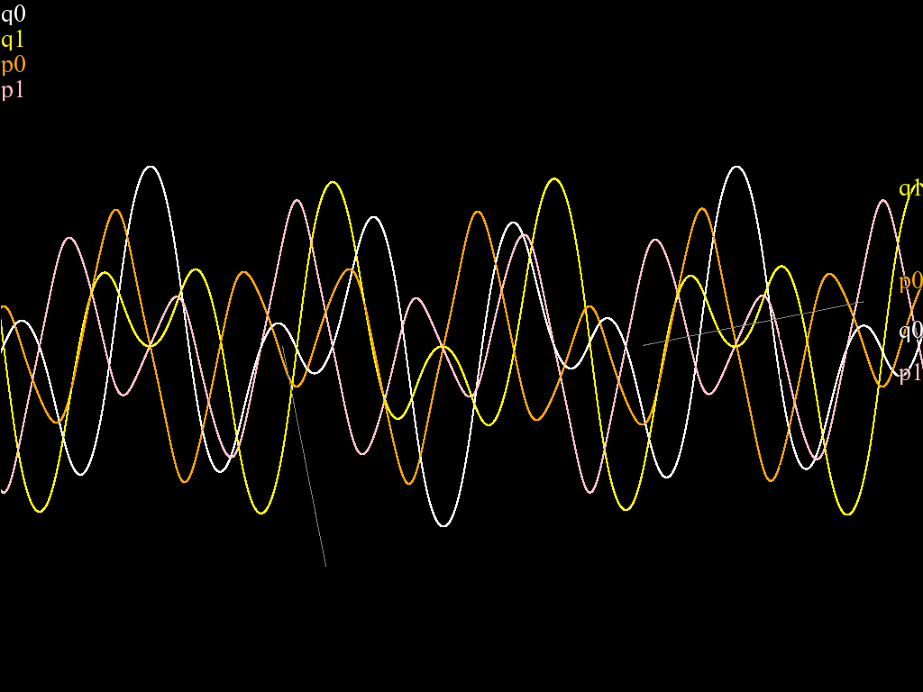
If you visit the page I have just created, you may find the simulation of a mechanical system.
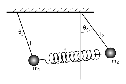
It is currently depicting two pendulum coupled with a spring (with and , and the original length of the spring is zero, and the two hanging points overlap),
which is a classical example of non-linearly coupled system.
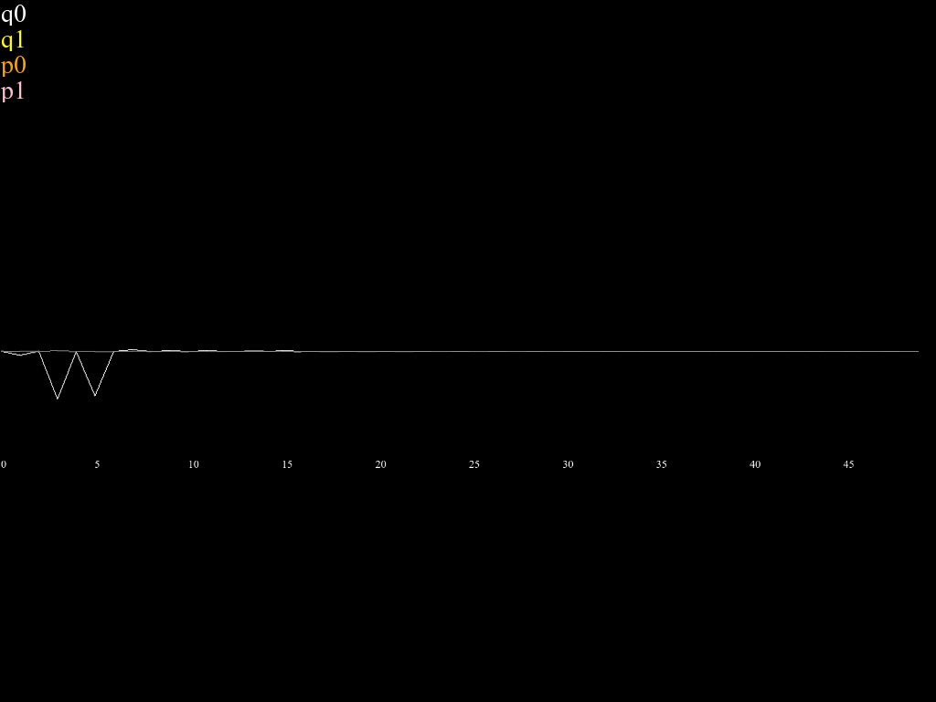
The pattern of the oscillation can be analyzed using discrete Fourier transformation, whose result can be found by clicking the buttons in the up-left corner (after the simulator has detected a period).
Hitting the space bar can make the simulation pause.
If you want to use it to simulate other mechanical systems, you can study the codes I wrote and write your own codes in the console.
By the way, the OpenRGSS version of the simulator is open-source here. Please star the repo if you like it.
]]>UlyssesZhanulysseszhan@gmail.comon web!]]><![CDATA[Simulating a mechanical system using RGSS3]]>2020-04-27T20:51:17-07:002020-04-27T20:51:17-07:00https://ulysseszh.github.io/physics/2020/04/28/simulation-rgssOur goal is to simulate a mechanical system according to its Hamiltonian .
To utilize the canonical equations we need to calculate the partial derivatives of . Here is a simple code to calculate partial derivatives.
(RGSS do not have matrix.rb, you can copy one from the attached file below.) Here x0 is a Vector, f is a call-able object as a function of vectors, dx is a small scalar which we are going to take 1e-6.
Let x = Vector[*q, *p], and then Formula 1 has the form To solve this equation numerically, we need to use a famous method called the (explicit) Runge–Kutta method.
The codes are not complete in this post. See the attached file for details. You can open the project using RPG Maker VX Ace. The Game.exe file is not the official Game.exe executable but the third-party improved version of it called RGD (of version 1.3.2, while the latest till now is 1.5.1).
]]>UlyssesZhanulysseszhan@gmail.com<![CDATA[The concentration change of gas in reversible reactions]]>2020-04-11T19:00:01-07:002020-04-11T19:00:01-07:00https://ulysseszh.github.io/chemistry/2020/04/12/concentration-timeIntroduction
A reversible elementary reaction takes place inside a closed, highly thermally conductive container of constant volume, whose reactants are all gases, and the reaction equation is where and are reactants, and and are stoichiometries.
Use square brackets to denote concentrations. Our goal is to find and as functions with respect to time .
The approach
It is easy to write out the rate equations where and are rate constants derived by experimenting.
Apply a substitution to Formula 1, and then it becomes which means the changes of are all equal, the changes of are all equal, and the changes of are opposite to the changes of .
Denote the changes of are equal to , the initial value of is , the initial value of is , which means Substitute Formula 4 into Formula 3, and it can be derived that by which we can reduce the problem to an integral problem where is a polynomial of th degree, where is the larger of the orders of the forward and reverse reactions. The degree of may be lower if the high-order term is offset, but only mathematicians believe in such coincidences.
Since Formula 5 is to integrate a rational function, it is easy.
After deriving as a function of , substitute it into Formula 4 and then Formula 2. We can derive as the answer.
Properties of
As we all know, here exists a state where the system is in chemical equilibrium. Denote the value of in this case as . It is easy to figure out that is a zero of on the interval which is the range of such that the concentration of all reactants are positive.
It is obvious that the value of is unique. It is because is monotonic over and the signs of its value at ends of interval are different.
Note that is a flaw of and that the improper integral diverges, so we can imagine how changes with respect to . when , and then changes monotonically, and finally when . Thus, the range of over
is for or for . is not considered because only mathematicians believe in such coincidences.
Suppose has different complex zeros , one of which is . The possible existence of multiple roots is ignored because only mathematicians believe in such coincidences. Decompose the rational function into several partial fractions, and it can be derived that where are undetermined coefficients.
Integrate Formula 8, and then it can be derived that In most cases, Formula 9 cannot be solved analytically and can only be solved numerically.
Note that if the coefficients are in general commensurable, Formula 9 can be reduced into a rational equation. However, only mathematicians believe in such coincidences. However, if , it can be proved that the equation can be reduced into a rational one.
Example
The closed container that is highly thermally conductive is in a certain temperature environment, and the water-gas shift reaction occurs under the catalysis of a certain catalyst, where the forward rate constant and the reverse rate constant Initial concentrations are Find
as a function of time.
Formula 6 becomes It is a polynomial of nd degree. Its two roots are Decomposing into partial fractions, we can derive that Thus, Since and are in general commensurable, we can solve the equation analytically into Use Formula 7, and then we can find the answer