<?xml version="1.0" encoding="utf-8"?><feed xmlns="http://www.w3.org/2005/Atom" xml:lang="en-US"><generator uri="https://jekyllrb.com/" version="4.4.1">Jekyll</generator><link href="https://ulysseszh.github.io/feed/math.xml" rel="self" type="application/atom+xml" /><link href="https://ulysseszh.github.io/" rel="alternate" type="text/html" hreflang="en-US" /><updated>2026-04-30T17:49:58-07:00</updated><id>https://ulysseszh.github.io/feed/math.xml</id><title type="html"><![CDATA[Ulysses’ trip | Math]]></title><subtitle>Here we are at the awesome (awful) blog written by UlyssesZhan!</subtitle><author><name>UlyssesZhan</name><email>ulysseszhan@gmail.com</email></author><entry><title type="html"><![CDATA[Determining the stabilizability of the abelian sandpile model]]></title><link href="https://ulysseszh.github.io/math/2026/01/03/sandpile-stabilizable.html" rel="alternate" type="text/html" title="Determining the stabilizability of the abelian sandpile model" /><published>2026-01-03T14:56:49-08:00</published><updated>2026-01-03T14:56:49-08:00</updated><id>https://ulysseszh.github.io/math/2026/01/03/sandpile-stabilizable</id><content type="html" xml:base="https://ulysseszh.github.io/math/2026/01/03/sandpile-stabilizable.html"><![CDATA[<h2 data-label="0.1" id="introduction">Introduction</h2>
<p>Suppose that we have <span class="katex"><span class="katex-mathml"><math xmlns="http://www.w3.org/1998/Math/MathML"><semantics><mrow><mi>n</mi></mrow><annotation encoding="application/x-tex">n</annotation></semantics></math></span></span> sandpiles denoted as a set <span class="katex"><span class="katex-mathml"><math xmlns="http://www.w3.org/1998/Math/MathML"><semantics><mrow><mi>V</mi></mrow><annotation encoding="application/x-tex">V</annotation></semantics></math></span></span>. Each sandpile <span class="katex"><span class="katex-mathml"><math xmlns="http://www.w3.org/1998/Math/MathML"><semantics><mrow><mi>x</mi><mo>∈</mo><mi>V</mi></mrow><annotation encoding="application/x-tex">x\in V</annotation></semantics></math></span></span> has a <dfn>toppling threshold</dfn> <span class="katex"><span class="katex-mathml"><math xmlns="http://www.w3.org/1998/Math/MathML"><semantics><mrow><mi>θ</mi><mtext> ⁣</mtext><mrow><mo fence="true">(</mo><mi>x</mi><mo fence="true">)</mo></mrow><mo>∈</mo><msub><mi mathvariant="double-struck">R</mi><mrow><mo>&gt;</mo><mn>0</mn></mrow></msub></mrow><annotation encoding="application/x-tex">\fc\tht x\in\bR_{&gt;0}</annotation></semantics></math></span></span>, and each ordered pair of sandpiles <span class="katex"><span class="katex-mathml"><math xmlns="http://www.w3.org/1998/Math/MathML"><semantics><mrow><mi>x</mi><mo separator="true">,</mo><msup><mi>x</mi><mo mathvariant="normal" lspace="0em" rspace="0em">′</mo></msup><mo>∈</mo><mi>V</mi></mrow><annotation encoding="application/x-tex">x,x'\in V</annotation></semantics></math></span></span> has a <dfn>toppling transfer amount</dfn> <span class="katex"><span class="katex-mathml"><math xmlns="http://www.w3.org/1998/Math/MathML"><semantics><mrow><mi>α</mi><mtext> ⁣</mtext><mrow><mo fence="true">(</mo><mi>x</mi><mo separator="true">,</mo><msup><mi>x</mi><mo mathvariant="normal" lspace="0em" rspace="0em">′</mo></msup><mo fence="true">)</mo></mrow><mo>∈</mo><msub><mi mathvariant="double-struck">R</mi><mrow><mo>≥</mo><mn>0</mn></mrow></msub></mrow><annotation encoding="application/x-tex">\fc\alp{x,x'}\in\bR_{\ge0}</annotation></semantics></math></span></span>. The tuple <span class="katex"><span class="katex-mathml"><math xmlns="http://www.w3.org/1998/Math/MathML"><semantics><mrow><mo fence="true">(</mo><mi>V</mi><mo separator="true">,</mo><mi>θ</mi><mo separator="true">,</mo><mi>α</mi><mo fence="true">)</mo></mrow><annotation encoding="application/x-tex">\p{V,\tht,\alp}</annotation></semantics></math></span></span> is called an <dfn>abelian sandpile model</dfn>.</p>
<p>A <dfn>configuration</dfn> <span class="katex"><span class="katex-mathml"><math xmlns="http://www.w3.org/1998/Math/MathML"><semantics><mrow><mi>η</mi><mo>:</mo><mi>x</mi><mo>→</mo><mi mathvariant="double-struck">R</mi></mrow><annotation encoding="application/x-tex">\eta:x\to\bR</annotation></semantics></math></span></span> is to assign an amount of sand <span class="katex"><span class="katex-mathml"><math xmlns="http://www.w3.org/1998/Math/MathML"><semantics><mrow><mi>η</mi><mtext> ⁣</mtext><mrow><mo fence="true">(</mo><mi>x</mi><mo fence="true">)</mo></mrow></mrow><annotation encoding="application/x-tex">\fc\eta x</annotation></semantics></math></span></span> to each sandpile <span class="katex"><span class="katex-mathml"><math xmlns="http://www.w3.org/1998/Math/MathML"><semantics><mrow><mi>x</mi><mo>∈</mo><mi>V</mi></mrow><annotation encoding="application/x-tex">x\in V</annotation></semantics></math></span></span>, and it is <dfn>legal</dfn> if <span class="katex"><span class="katex-mathml"><math xmlns="http://www.w3.org/1998/Math/MathML"><semantics><mrow><mi>η</mi><mtext> ⁣</mtext><mrow><mo fence="true">(</mo><mi>x</mi><mo fence="true">)</mo></mrow><mo>≥</mo><mn>0</mn></mrow><annotation encoding="application/x-tex">\fc\eta x\ge0</annotation></semantics></math></span></span> for all <span class="katex"><span class="katex-mathml"><math xmlns="http://www.w3.org/1998/Math/MathML"><semantics><mrow><mi>x</mi><mo>∈</mo><mi>V</mi></mrow><annotation encoding="application/x-tex">x\in V</annotation></semantics></math></span></span> (or conveniently denoted as <span class="katex"><span class="katex-mathml"><math xmlns="http://www.w3.org/1998/Math/MathML"><semantics><mrow><mi>η</mi><mo>≥</mo><mn>0</mn></mrow><annotation encoding="application/x-tex">\eta\ge0</annotation></semantics></math></span></span>). For any configuration <span class="katex"><span class="katex-mathml"><math xmlns="http://www.w3.org/1998/Math/MathML"><semantics><mrow><mi>η</mi></mrow><annotation encoding="application/x-tex">\eta</annotation></semantics></math></span></span>, any <span class="katex"><span class="katex-mathml"><math xmlns="http://www.w3.org/1998/Math/MathML"><semantics><mrow><mi>y</mi><mo>∈</mo><mi>V</mi></mrow><annotation encoding="application/x-tex">y\in V</annotation></semantics></math></span></span> can <dfn>topple</dfn>, which is a transition to a new configuration <span class="katex"><span class="katex-mathml"><math xmlns="http://www.w3.org/1998/Math/MathML"><semantics><mrow><msup><mi>η</mi><mo mathvariant="normal" lspace="0em" rspace="0em">′</mo></msup></mrow><annotation encoding="application/x-tex">\eta'</annotation></semantics></math></span></span> defined as
<span class="katex-display"><span class="katex"><span class="katex-mathml"><math xmlns="http://www.w3.org/1998/Math/MathML" display="block"><semantics><mrow><msup><mi>η</mi><mo mathvariant="normal" lspace="0em" rspace="0em">′</mo></msup><mtext> ⁣</mtext><mrow><mo fence="true">(</mo><mi>x</mi><mo fence="true">)</mo></mrow><mo><mi mathvariant="normal">≔</mi></mo><mi>η</mi><mtext> ⁣</mtext><mrow><mo fence="true">(</mo><mi>x</mi><mo fence="true">)</mo></mrow><mo>−</mo><mi>θ</mi><mtext> ⁣</mtext><mrow><mo fence="true">(</mo><mi>y</mi><mo fence="true">)</mo></mrow><msub><mi>δ</mi><mrow><mi>x</mi><mi>y</mi></mrow></msub><mo>+</mo><mi>α</mi><mtext> ⁣</mtext><mrow><mo fence="true">(</mo><mi>y</mi><mo separator="true">,</mo><mi>x</mi><mo fence="true">)</mo></mrow><mi mathvariant="normal">.</mi></mrow><annotation encoding="application/x-tex">\fc{\eta'}x\ceq\fc\eta x-\fc\tht y\dlt_{xy}+\fc\alp{y,x}.</annotation></semantics></math></span></span></span> The toppling is <dfn>legal</dfn> if <span class="katex"><span class="katex-mathml"><math xmlns="http://www.w3.org/1998/Math/MathML"><semantics><mrow><mi>η</mi><mtext> ⁣</mtext><mrow><mo fence="true">(</mo><mi>y</mi><mo fence="true">)</mo></mrow><mo>≥</mo><mi>θ</mi><mtext> ⁣</mtext><mrow><mo fence="true">(</mo><mi>y</mi><mo fence="true">)</mo></mrow></mrow><annotation encoding="application/x-tex">\fc\eta y\ge\fc\tht y</annotation></semantics></math></span></span>, in which case we call <span class="katex"><span class="katex-mathml"><math xmlns="http://www.w3.org/1998/Math/MathML"><semantics><mrow><mi>y</mi></mrow><annotation encoding="application/x-tex">y</annotation></semantics></math></span></span> an <dfn>unstable</dfn> site of the configuration <span class="katex"><span class="katex-mathml"><math xmlns="http://www.w3.org/1998/Math/MathML"><semantics><mrow><mi>η</mi></mrow><annotation encoding="application/x-tex">\eta</annotation></semantics></math></span></span>. Notice that a legal configuration undergoing a legal toppling must become a legal configuration. A sequence of topplings where each toppling uses the resultant configuration of the previous toppling as the initial configuration is called a <dfn>toppling procedure</dfn>.</p>
<p>In its historically original form (<a href="https://doi.org/10.1103/PhysRevLett.64.1613" target="_blank" rel="external">Dhar, 1990</a>), <span class="katex"><span class="katex-mathml"><math xmlns="http://www.w3.org/1998/Math/MathML"><semantics><mrow><mi>V</mi></mrow><annotation encoding="application/x-tex">V</annotation></semantics></math></span></span> is the lattice sites on a 2D rectangular grid, and <span class="katex"><span class="katex-mathml"><math xmlns="http://www.w3.org/1998/Math/MathML"><semantics><mrow><mi>θ</mi><mtext> ⁣</mtext><mrow><mo fence="true">(</mo><mi>x</mi><mo fence="true">)</mo></mrow><mo>=</mo><mn>4</mn></mrow><annotation encoding="application/x-tex">\fc\tht x=4</annotation></semantics></math></span></span> for all <span class="katex"><span class="katex-mathml"><math xmlns="http://www.w3.org/1998/Math/MathML"><semantics><mrow><mi>x</mi><mo>∈</mo><mi>V</mi></mrow><annotation encoding="application/x-tex">x\in V</annotation></semantics></math></span></span>, and <span class="katex"><span class="katex-mathml"><math xmlns="http://www.w3.org/1998/Math/MathML"><semantics><mrow><mi>α</mi><mtext> ⁣</mtext><mrow><mo fence="true">(</mo><mi>x</mi><mo separator="true">,</mo><msup><mi>x</mi><mo mathvariant="normal" lspace="0em" rspace="0em">′</mo></msup><mo fence="true">)</mo></mrow></mrow><annotation encoding="application/x-tex">\fc\alp{x,x'}</annotation></semantics></math></span></span> is <span class="katex"><span class="katex-mathml"><math xmlns="http://www.w3.org/1998/Math/MathML"><semantics><mrow><mn>1</mn></mrow><annotation encoding="application/x-tex">1</annotation></semantics></math></span></span> if <span class="katex"><span class="katex-mathml"><math xmlns="http://www.w3.org/1998/Math/MathML"><semantics><mrow><mi>x</mi></mrow><annotation encoding="application/x-tex">x</annotation></semantics></math></span></span> and <span class="katex"><span class="katex-mathml"><math xmlns="http://www.w3.org/1998/Math/MathML"><semantics><mrow><msup><mi>x</mi><mo mathvariant="normal" lspace="0em" rspace="0em">′</mo></msup></mrow><annotation encoding="application/x-tex">x'</annotation></semantics></math></span></span> are nearest neighbors or <span class="katex"><span class="katex-mathml"><math xmlns="http://www.w3.org/1998/Math/MathML"><semantics><mrow><mn>0</mn></mrow><annotation encoding="application/x-tex">0</annotation></semantics></math></span></span> otherwise. It is then generalized to an arbitrary directed multigraph (<a href="https://doi.org/10.1007/978-3-7643-8786-0_17" target="_blank" rel="external">Holroyd et al., 2008</a>), where <span class="katex"><span class="katex-mathml"><math xmlns="http://www.w3.org/1998/Math/MathML"><semantics><mrow><mi>V</mi></mrow><annotation encoding="application/x-tex">V</annotation></semantics></math></span></span> is its vertices, and <span class="katex"><span class="katex-mathml"><math xmlns="http://www.w3.org/1998/Math/MathML"><semantics><mrow><mi>θ</mi><mtext> ⁣</mtext><mrow><mo fence="true">(</mo><mi>x</mi><mo fence="true">)</mo></mrow></mrow><annotation encoding="application/x-tex">\fc\tht x</annotation></semantics></math></span></span> is the out-degree of vertex <span class="katex"><span class="katex-mathml"><math xmlns="http://www.w3.org/1998/Math/MathML"><semantics><mrow><mi>x</mi></mrow><annotation encoding="application/x-tex">x</annotation></semantics></math></span></span>, and <span class="katex"><span class="katex-mathml"><math xmlns="http://www.w3.org/1998/Math/MathML"><semantics><mrow><mi>α</mi><mtext> ⁣</mtext><mrow><mo fence="true">(</mo><mi>x</mi><mo separator="true">,</mo><msup><mi>x</mi><mo mathvariant="normal" lspace="0em" rspace="0em">′</mo></msup><mo fence="true">)</mo></mrow></mrow><annotation encoding="application/x-tex">\fc\alp{x,x'}</annotation></semantics></math></span></span> is the number of edges from <span class="katex"><span class="katex-mathml"><math xmlns="http://www.w3.org/1998/Math/MathML"><semantics><mrow><mi>x</mi></mrow><annotation encoding="application/x-tex">x</annotation></semantics></math></span></span> to
<span class="katex"><span class="katex-mathml"><math xmlns="http://www.w3.org/1998/Math/MathML"><semantics><mrow><msup><mi>x</mi><mo mathvariant="normal" lspace="0em" rspace="0em">′</mo></msup></mrow><annotation encoding="application/x-tex">x'</annotation></semantics></math></span></span>.</p>
<p>A configuration where none of the sandpiles can legally topple is called a <dfn>stable</dfn> configuration. In other words, configuration <span class="katex"><span class="katex-mathml"><math xmlns="http://www.w3.org/1998/Math/MathML"><semantics><mrow><mi>η</mi></mrow><annotation encoding="application/x-tex">\eta</annotation></semantics></math></span></span> is stable if <span class="katex"><span class="katex-mathml"><math xmlns="http://www.w3.org/1998/Math/MathML"><semantics><mrow><mi>η</mi><mtext> ⁣</mtext><mrow><mo fence="true">(</mo><mi>x</mi><mo fence="true">)</mo></mrow><mo>&lt;</mo><mi>θ</mi><mtext> ⁣</mtext><mrow><mo fence="true">(</mo><mi>x</mi><mo fence="true">)</mo></mrow></mrow><annotation encoding="application/x-tex">\fc\eta x&lt;\fc\tht x</annotation></semantics></math></span></span> for all <span class="katex"><span class="katex-mathml"><math xmlns="http://www.w3.org/1998/Math/MathML"><semantics><mrow><mi>x</mi><mo>∈</mo><mi>V</mi></mrow><annotation encoding="application/x-tex">x\in V</annotation></semantics></math></span></span>, or denoted as <span class="katex"><span class="katex-mathml"><math xmlns="http://www.w3.org/1998/Math/MathML"><semantics><mrow><mi>η</mi><mo>&lt;</mo><mi>θ</mi></mrow><annotation encoding="application/x-tex">\eta&lt;\tht</annotation></semantics></math></span></span> in abbreviation. A toppling procedure that makes a configuration stable is called a <dfn>stabilizing</dfn> toppling procedure that stabilizes the configuration. A legal configuration is <dfn>stabilizable</dfn> if it has a finite legal stabilizing toppling procedure. Otherwise, the configuration is <dfn>exploding</dfn>. A natural question to ask then is how to determine whether a configuration is stabilizable or exploding.</p>
<h2 data-label="0.2" id="abelian-property">Abelian property</h2>
<p>One important fact to notice is that the abelian sandpile model has the so-called <dfn>abelian property</dfn>: if a configuration is stabilizable, then every legal toppling procedure of it is finite, and the stabilizing legal toppling procedure is unique up to the order of topplings. In other words, if we define the <dfn>toppling counting function</dfn> <span class="katex"><span class="katex-mathml"><math xmlns="http://www.w3.org/1998/Math/MathML"><semantics><mrow><mi>u</mi><mo>:</mo><mi>V</mi><mo>→</mo><mi mathvariant="double-struck">N</mi></mrow><annotation encoding="application/x-tex">u:V\to\bN</annotation></semantics></math></span></span> such that <span class="katex"><span class="katex-mathml"><math xmlns="http://www.w3.org/1998/Math/MathML"><semantics><mrow><mi>u</mi><mtext> ⁣</mtext><mrow><mo fence="true">(</mo><mi>x</mi><mo fence="true">)</mo></mrow></mrow><annotation encoding="application/x-tex">\fc ux</annotation></semantics></math></span></span> is the number of times that <span class="katex"><span class="katex-mathml"><math xmlns="http://www.w3.org/1998/Math/MathML"><semantics><mrow><mi>x</mi><mo>∈</mo><mi>V</mi></mrow><annotation encoding="application/x-tex">x\in V</annotation></semantics></math></span></span> topples throughout the toppling procedure, then every legal stabilizing toppling procedure of a stabilizable configuration has the same toppling counting function, which is called the <dfn>odometer</dfn> of the configuration. We will leave the proof of the abelian property to a later part in this section.</p>
<p>In order to better describe the model, we can define a function <span class="katex"><span class="katex-mathml"><math xmlns="http://www.w3.org/1998/Math/MathML"><semantics><mrow><mi mathvariant="normal">Δ</mi><mo>:</mo><mi>V</mi><mo>×</mo><mi>V</mi><mo>→</mo><mi mathvariant="double-struck">R</mi></mrow><annotation encoding="application/x-tex">\Dlt:V\times V\to\bR</annotation></semantics></math></span></span> (the notation comes from the notation of the Laplacian operator in vector analysis due to its direct analogy in the case of the abelian sandpile model on a grid, in which case it is called a Laplacian matrix in the language of graph theory) as follows: <span class="katex-display"><span class="katex"><span class="katex-mathml"><math xmlns="http://www.w3.org/1998/Math/MathML" display="block"><semantics><mrow><mi mathvariant="normal">Δ</mi><mtext> ⁣</mtext><mrow><mo fence="true">(</mo><mi>x</mi><mo separator="true">,</mo><mi>y</mi><mo fence="true">)</mo></mrow><mo>=</mo><mi>θ</mi><mtext> ⁣</mtext><mrow><mo fence="true">(</mo><mi>x</mi><mo fence="true">)</mo></mrow><msub><mi>δ</mi><mrow><mi>x</mi><mi>y</mi></mrow></msub><mo>−</mo><mi>α</mi><mtext> ⁣</mtext><mrow><mo fence="true">(</mo><mi>x</mi><mo separator="true">,</mo><mi>y</mi><mo fence="true">)</mo></mrow><mi mathvariant="normal">.</mi></mrow><annotation encoding="application/x-tex">\fc\Dlt{x,y}=\fc\tht x\dlt_{xy}-\fc\alp{x,y}.</annotation></semantics></math></span></span></span> It encodes information from both <span class="katex"><span class="katex-mathml"><math xmlns="http://www.w3.org/1998/Math/MathML"><semantics><mrow><mi>θ</mi></mrow><annotation encoding="application/x-tex">\tht</annotation></semantics></math></span></span> and <span class="katex"><span class="katex-mathml"><math xmlns="http://www.w3.org/1998/Math/MathML"><semantics><mrow><mi>α</mi></mrow><annotation encoding="application/x-tex">\alp</annotation></semantics></math></span></span> and provides everything we need to know to find the resultant configuration given any initial configuration and the toppling counting function. Explicitly, configuration <span class="katex"><span class="katex-mathml"><math xmlns="http://www.w3.org/1998/Math/MathML"><semantics><mrow><mi>η</mi></mrow><annotation encoding="application/x-tex">\eta</annotation></semantics></math></span></span> undergoing a toppling procedure with the toppling counting function <span class="katex"><span class="katex-mathml"><math xmlns="http://www.w3.org/1998/Math/MathML"><semantics><mrow><mi>u</mi></mrow><annotation encoding="application/x-tex">u</annotation></semantics></math></span></span> becomes
<span class="katex-display"><span class="katex"><span class="katex-mathml"><math xmlns="http://www.w3.org/1998/Math/MathML" display="block"><semantics><mrow><msup><mi>η</mi><mo mathvariant="normal" lspace="0em" rspace="0em">′</mo></msup><mtext> ⁣</mtext><mrow><mo fence="true">(</mo><mi>x</mi><mo fence="true">)</mo></mrow><mo>=</mo><mi>η</mi><mtext> ⁣</mtext><mrow><mo fence="true">(</mo><mi>x</mi><mo fence="true">)</mo></mrow><mo>−</mo><munder><mo>∑</mo><mi>y</mi></munder><mi mathvariant="normal">Δ</mi><mtext> ⁣</mtext><mrow><mo fence="true">(</mo><mi>x</mi><mo separator="true">,</mo><mi>y</mi><mo fence="true">)</mo></mrow><mi>u</mi><mtext> ⁣</mtext><mrow><mo fence="true">(</mo><mi>y</mi><mo fence="true">)</mo></mrow><mi mathvariant="normal">.</mi></mrow><annotation encoding="application/x-tex">\fc{\eta'}x=\fc\eta x-\sum_y\fc\Dlt{x,y}\fc uy.</annotation></semantics></math></span></span></span> For abbreviation, we denote <span class="katex"><span class="katex-mathml"><math xmlns="http://www.w3.org/1998/Math/MathML"><semantics><mrow><mi>x</mi><mo>↦</mo><msub><mo>∑</mo><mi>y</mi></msub><mi mathvariant="normal">Δ</mi><mtext> ⁣</mtext><mrow><mo fence="true">(</mo><mi>x</mi><mo separator="true">,</mo><mi>y</mi><mo fence="true">)</mo></mrow><mi>u</mi><mtext> ⁣</mtext><mrow><mo fence="true">(</mo><mi>y</mi><mo fence="true">)</mo></mrow></mrow><annotation encoding="application/x-tex">x\mapsto\sum_y\fc\Dlt{x,y}\fc uy</annotation></semantics></math></span></span> as <span class="katex"><span class="katex-mathml"><math xmlns="http://www.w3.org/1998/Math/MathML"><semantics><mrow><mi mathvariant="normal">Δ</mi><mi>u</mi></mrow><annotation encoding="application/x-tex">\Dlt u</annotation></semantics></math></span></span> so that
<span class="katex"><span class="katex-mathml"><math xmlns="http://www.w3.org/1998/Math/MathML"><semantics><mrow><mi mathvariant="normal">Δ</mi><mi>u</mi><mtext> ⁣</mtext><mrow><mo fence="true">(</mo><mi>x</mi><mo fence="true">)</mo></mrow><mo>=</mo><msub><mo>∑</mo><mi>y</mi></msub><mi mathvariant="normal">Δ</mi><mtext> ⁣</mtext><mrow><mo fence="true">(</mo><mi>x</mi><mo separator="true">,</mo><mi>y</mi><mo fence="true">)</mo></mrow><mi>u</mi><mtext> ⁣</mtext><mrow><mo fence="true">(</mo><mi>y</mi><mo fence="true">)</mo></mrow></mrow><annotation encoding="application/x-tex">\fc{\Dlt u}x=\sum_y\fc\Dlt{x,y}\fc uy</annotation></semantics></math></span></span>. Therefore, the resultant configuration of a toppling procedure can be denoted as <span class="katex"><span class="katex-mathml"><math xmlns="http://www.w3.org/1998/Math/MathML"><semantics><mrow><msup><mi>η</mi><mo mathvariant="normal" lspace="0em" rspace="0em">′</mo></msup><mo>=</mo><mi>η</mi><mo>−</mo><mi mathvariant="normal">Δ</mi><mi>u</mi></mrow><annotation encoding="application/x-tex">\eta'=\eta-\Dlt u</annotation></semantics></math></span></span>. This notation is natural if we think of <span class="katex"><span class="katex-mathml"><math xmlns="http://www.w3.org/1998/Math/MathML"><semantics><mrow><mi mathvariant="normal">Δ</mi></mrow><annotation encoding="application/x-tex">\Dlt</annotation></semantics></math></span></span> as an <span class="katex"><span class="katex-mathml"><math xmlns="http://www.w3.org/1998/Math/MathML"><semantics><mrow><mi>n</mi></mrow><annotation encoding="application/x-tex">n</annotation></semantics></math></span></span>-dimensional matrix and think of <span class="katex"><span class="katex-mathml"><math xmlns="http://www.w3.org/1998/Math/MathML"><semantics><mrow><mi>η</mi></mrow><annotation encoding="application/x-tex">\eta</annotation></semantics></math></span></span> and <span class="katex"><span class="katex-mathml"><math xmlns="http://www.w3.org/1998/Math/MathML"><semantics><mrow><mi>u</mi></mrow><annotation encoding="application/x-tex">u</annotation></semantics></math></span></span> as <span class="katex"><span class="katex-mathml"><math xmlns="http://www.w3.org/1998/Math/MathML"><semantics><mrow><mi>n</mi></mrow><annotation encoding="application/x-tex">n</annotation></semantics></math></span></span>-dimensional column vectors. This equation tells us that the resultant configuration of two toppling procedures is the same as long as they have the same toppling counting function.</p>
<p>A toppling procedure can then be expressed as a sequence of toppling counting functions where the <span class="katex"><span class="katex-mathml"><math xmlns="http://www.w3.org/1998/Math/MathML"><semantics><mrow><mi>t</mi></mrow><annotation encoding="application/x-tex">t</annotation></semantics></math></span></span>th toppling counting function <span class="katex"><span class="katex-mathml"><math xmlns="http://www.w3.org/1998/Math/MathML"><semantics><mrow><msub><mi>u</mi><mi>t</mi></msub></mrow><annotation encoding="application/x-tex">u_t</annotation></semantics></math></span></span> is that of the toppling procedure derived by truncating the full toppling procedure up to the first <span class="katex"><span class="katex-mathml"><math xmlns="http://www.w3.org/1998/Math/MathML"><semantics><mrow><mi>t</mi></mrow><annotation encoding="application/x-tex">t</annotation></semantics></math></span></span> topplings. If the <span class="katex"><span class="katex-mathml"><math xmlns="http://www.w3.org/1998/Math/MathML"><semantics><mrow><mi>t</mi></mrow><annotation encoding="application/x-tex">t</annotation></semantics></math></span></span>th toppling happens at site <span class="katex"><span class="katex-mathml"><math xmlns="http://www.w3.org/1998/Math/MathML"><semantics><mrow><mi>y</mi></mrow><annotation encoding="application/x-tex">y</annotation></semantics></math></span></span>, then <span class="katex-display"><span class="katex"><span class="katex-mathml"><math xmlns="http://www.w3.org/1998/Math/MathML" display="block"><semantics><mrow><msub><mi>u</mi><mi>t</mi></msub><mtext> ⁣</mtext><mrow><mo fence="true">(</mo><mi>x</mi><mo fence="true">)</mo></mrow><mo>−</mo><msub><mi>u</mi><mrow><mi>t</mi><mo>−</mo><mn>1</mn></mrow></msub><mtext> ⁣</mtext><mrow><mo fence="true">(</mo><mi>x</mi><mo fence="true">)</mo></mrow><mo>=</mo><msub><mi>δ</mi><mrow><mi>x</mi><mi>y</mi></mrow></msub><mi mathvariant="normal">.</mi></mrow><annotation encoding="application/x-tex">\fc{u_t}x-\fc{u_{t-1}}x=\dlt_{xy}.</annotation></semantics></math></span></span></span> We stipulate that <span class="katex"><span class="katex-mathml"><math xmlns="http://www.w3.org/1998/Math/MathML"><semantics><mrow><msub><mi>u</mi><mn>0</mn></msub></mrow><annotation encoding="application/x-tex">u_0</annotation></semantics></math></span></span> is the zero function. From now on, we call a sequence <span class="katex"><span class="katex-mathml"><math xmlns="http://www.w3.org/1998/Math/MathML"><semantics><mrow><msubsup><mrow><mo fence="true">{</mo><msub><mi>u</mi><mi>t</mi></msub><mo fence="true">}</mo></mrow><mrow><mi>t</mi><mo>=</mo><mn>0</mn></mrow><mi>T</mi></msubsup></mrow><annotation encoding="application/x-tex">\B{u_t}_{t=0}^T</annotation></semantics></math></span></span> (where
<span class="katex"><span class="katex-mathml"><math xmlns="http://www.w3.org/1998/Math/MathML"><semantics><mrow><mi>T</mi></mrow><annotation encoding="application/x-tex">T</annotation></semantics></math></span></span> is either a natural number or infinity) as a toppling procedure as long as the following conditions are satisfied: <span class="katex"><span class="katex-mathml"><math xmlns="http://www.w3.org/1998/Math/MathML"><semantics><mrow><msub><mi>u</mi><mn>0</mn></msub><mo>=</mo><mn>0</mn></mrow><annotation encoding="application/x-tex">u_0=0</annotation></semantics></math></span></span>, and for all <span class="katex"><span class="katex-mathml"><math xmlns="http://www.w3.org/1998/Math/MathML"><semantics><mrow><mn>0</mn><mo>≤</mo><mi>t</mi><mo>&lt;</mo><mi>T</mi></mrow><annotation encoding="application/x-tex">0\le t&lt;T</annotation></semantics></math></span></span>, there exists <span class="katex"><span class="katex-mathml"><math xmlns="http://www.w3.org/1998/Math/MathML"><semantics><mrow><mi>y</mi><mo>∈</mo><mi>V</mi></mrow><annotation encoding="application/x-tex">y\in V</annotation></semantics></math></span></span> such that <span class="katex"><span class="katex-mathml"><math xmlns="http://www.w3.org/1998/Math/MathML"><semantics><mrow><msub><mi>u</mi><mrow><mi>t</mi><mo>+</mo><mn>1</mn></mrow></msub><mtext> ⁣</mtext><mrow><mo fence="true">(</mo><mi>x</mi><mo fence="true">)</mo></mrow><mo>=</mo><msub><mi>u</mi><mi>t</mi></msub><mtext> ⁣</mtext><mrow><mo fence="true">(</mo><mi>x</mi><mo fence="true">)</mo></mrow><mo>+</mo><msub><mi>δ</mi><mrow><mi>x</mi><mi>y</mi></mrow></msub></mrow><annotation encoding="application/x-tex">\fc{u_{t+1}}x=\fc{u_t}x+\dlt_{xy}</annotation></semantics></math></span></span>. It is obvious to see that <span class="katex"><span class="katex-mathml"><math xmlns="http://www.w3.org/1998/Math/MathML"><semantics><mrow><msub><mo>∑</mo><mi>x</mi></msub><msub><mi>u</mi><mi>t</mi></msub><mtext> ⁣</mtext><mrow><mo fence="true">(</mo><mi>x</mi><mo fence="true">)</mo></mrow><mo>=</mo><mi>t</mi></mrow><annotation encoding="application/x-tex">\sum_x\fc{u_t}x=t</annotation></semantics></math></span></span> for all
<span class="katex"><span class="katex-mathml"><math xmlns="http://www.w3.org/1998/Math/MathML"><semantics><mrow><mi>t</mi></mrow><annotation encoding="application/x-tex">t</annotation></semantics></math></span></span>. Therefore, the length <span class="katex"><span class="katex-mathml"><math xmlns="http://www.w3.org/1998/Math/MathML"><semantics><mrow><mi>T</mi></mrow><annotation encoding="application/x-tex">T</annotation></semantics></math></span></span> of a toppling procedure is the same as the sum <span class="katex"><span class="katex-mathml"><math xmlns="http://www.w3.org/1998/Math/MathML"><semantics><mrow><msub><mo>∑</mo><mi>x</mi></msub><mi>u</mi><mtext> ⁣</mtext><mrow><mo fence="true">(</mo><mi>x</mi><mo fence="true">)</mo></mrow></mrow><annotation encoding="application/x-tex">\sum_x\fc ux</annotation></semantics></math></span></span>, where <span class="katex"><span class="katex-mathml"><math xmlns="http://www.w3.org/1998/Math/MathML"><semantics><mrow><mi>u</mi><mo><mi mathvariant="normal">≔</mi></mo><msub><mi>u</mi><mi>T</mi></msub></mrow><annotation encoding="application/x-tex">u\ceq u_T</annotation></semantics></math></span></span> is the final toppling counting function of the toppling procedure. The definition of the legality of a toppling procedure is also naturally extended to this formulation.</p>
<p>Because the resultant configuration of a toppling procedure is independent of the order of the topplings, for two different sites <span class="katex"><span class="katex-mathml"><math xmlns="http://www.w3.org/1998/Math/MathML"><semantics><mrow><mi>y</mi></mrow><annotation encoding="application/x-tex">y</annotation></semantics></math></span></span> and <span class="katex"><span class="katex-mathml"><math xmlns="http://www.w3.org/1998/Math/MathML"><semantics><mrow><msup><mi>y</mi><mo mathvariant="normal" lspace="0em" rspace="0em">′</mo></msup></mrow><annotation encoding="application/x-tex">y'</annotation></semantics></math></span></span>, toppling <span class="katex"><span class="katex-mathml"><math xmlns="http://www.w3.org/1998/Math/MathML"><semantics><mrow><mi>y</mi></mrow><annotation encoding="application/x-tex">y</annotation></semantics></math></span></span> and then <span class="katex"><span class="katex-mathml"><math xmlns="http://www.w3.org/1998/Math/MathML"><semantics><mrow><msup><mi>y</mi><mo mathvariant="normal" lspace="0em" rspace="0em">′</mo></msup></mrow><annotation encoding="application/x-tex">y'</annotation></semantics></math></span></span> is equivalent to toppling <span class="katex"><span class="katex-mathml"><math xmlns="http://www.w3.org/1998/Math/MathML"><semantics><mrow><msup><mi>y</mi><mo mathvariant="normal" lspace="0em" rspace="0em">′</mo></msup></mrow><annotation encoding="application/x-tex">y'</annotation></semantics></math></span></span> and then <span class="katex"><span class="katex-mathml"><math xmlns="http://www.w3.org/1998/Math/MathML"><semantics><mrow><mi>y</mi></mrow><annotation encoding="application/x-tex">y</annotation></semantics></math></span></span>. Both toppling procedures have the same toppling counting function <span class="katex"><span class="katex-mathml"><math xmlns="http://www.w3.org/1998/Math/MathML"><semantics><mrow><msub><mi>δ</mi><mrow><mi>x</mi><mi>y</mi></mrow></msub><mo>+</mo><msub><mi>δ</mi><mrow><mi>x</mi><msup><mi>y</mi><mo mathvariant="normal" lspace="0em" rspace="0em">′</mo></msup></mrow></msub></mrow><annotation encoding="application/x-tex">\dlt_{xy}+\dlt_{xy'}</annotation></semantics></math></span></span>. If both sites are unstable sites of the initial configuration, then both toppling procedures are legal. To see this, suppose that <span class="katex"><span class="katex-mathml"><math xmlns="http://www.w3.org/1998/Math/MathML"><semantics><mrow><mi>y</mi></mrow><annotation encoding="application/x-tex">y</annotation></semantics></math></span></span> and <span class="katex"><span class="katex-mathml"><math xmlns="http://www.w3.org/1998/Math/MathML"><semantics><mrow><msup><mi>y</mi><mo mathvariant="normal" lspace="0em" rspace="0em">′</mo></msup></mrow><annotation encoding="application/x-tex">y'</annotation></semantics></math></span></span> are two different unstable sites of the configuration <span class="katex"><span class="katex-mathml"><math xmlns="http://www.w3.org/1998/Math/MathML"><semantics><mrow><mi>η</mi></mrow><annotation encoding="application/x-tex">\eta</annotation></semantics></math></span></span>. Then, the configuration <span class="katex"><span class="katex-mathml"><math xmlns="http://www.w3.org/1998/Math/MathML"><semantics><mrow><msup><mi>η</mi><mo mathvariant="normal" lspace="0em" rspace="0em">′</mo></msup></mrow><annotation encoding="application/x-tex">\eta'</annotation></semantics></math></span></span> after
<span class="katex"><span class="katex-mathml"><math xmlns="http://www.w3.org/1998/Math/MathML"><semantics><mrow><mi>y</mi></mrow><annotation encoding="application/x-tex">y</annotation></semantics></math></span></span> topples is given by <span class="katex"><span class="katex-mathml"><math xmlns="http://www.w3.org/1998/Math/MathML"><semantics><mrow><msup><mi>η</mi><mo mathvariant="normal" lspace="0em" rspace="0em">′</mo></msup><mtext> ⁣</mtext><mrow><mo fence="true">(</mo><mi>x</mi><mo fence="true">)</mo></mrow><mo>=</mo><mi>η</mi><mtext> ⁣</mtext><mrow><mo fence="true">(</mo><mi>x</mi><mo fence="true">)</mo></mrow><mo>−</mo><mi>θ</mi><mtext> ⁣</mtext><mrow><mo fence="true">(</mo><mi>y</mi><mo fence="true">)</mo></mrow><msub><mi>δ</mi><mrow><mi>x</mi><mi>y</mi></mrow></msub><mo>+</mo><mi>α</mi><mtext> ⁣</mtext><mrow><mo fence="true">(</mo><mi>y</mi><mo separator="true">,</mo><mi>x</mi><mo fence="true">)</mo></mrow></mrow><annotation encoding="application/x-tex">\fc{\eta'}x=\fc\eta x-\fc\tht y\dlt_{xy}+\fc\alp{y,x}</annotation></semantics></math></span></span>. Its value at <span class="katex"><span class="katex-mathml"><math xmlns="http://www.w3.org/1998/Math/MathML"><semantics><mrow><msup><mi>y</mi><mo mathvariant="normal" lspace="0em" rspace="0em">′</mo></msup></mrow><annotation encoding="application/x-tex">y'</annotation></semantics></math></span></span> is
<span class="katex"><span class="katex-mathml"><math xmlns="http://www.w3.org/1998/Math/MathML"><semantics><mrow><msup><mi>η</mi><mo mathvariant="normal" lspace="0em" rspace="0em">′</mo></msup><mtext> ⁣</mtext><mrow><mo fence="true">(</mo><msup><mi>y</mi><mo mathvariant="normal" lspace="0em" rspace="0em">′</mo></msup><mo fence="true">)</mo></mrow><mo>=</mo><mi>η</mi><mtext> ⁣</mtext><mrow><mo fence="true">(</mo><msup><mi>y</mi><mo mathvariant="normal" lspace="0em" rspace="0em">′</mo></msup><mo fence="true">)</mo></mrow><mo>+</mo><mi>α</mi><mtext> ⁣</mtext><mrow><mo fence="true">(</mo><mi>y</mi><mo separator="true">,</mo><msup><mi>y</mi><mo mathvariant="normal" lspace="0em" rspace="0em">′</mo></msup><mo fence="true">)</mo></mrow></mrow><annotation encoding="application/x-tex">\fc{\eta'}{y'}=\fc\eta{y'}+\fc\alp{y,y'}</annotation></semantics></math></span></span> (notice that <span class="katex"><span class="katex-mathml"><math xmlns="http://www.w3.org/1998/Math/MathML"><semantics><mrow><msub><mi>δ</mi><mrow><mi>y</mi><msup><mi>y</mi><mo mathvariant="normal" lspace="0em" rspace="0em">′</mo></msup></mrow></msub><mo>=</mo><mn>0</mn></mrow><annotation encoding="application/x-tex">\dlt_{yy'}=0</annotation></semantics></math></span></span> because <span class="katex"><span class="katex-mathml"><math xmlns="http://www.w3.org/1998/Math/MathML"><semantics><mrow><mi>y</mi><mo mathvariant="normal">≠</mo><msup><mi>y</mi><mo mathvariant="normal" lspace="0em" rspace="0em">′</mo></msup></mrow><annotation encoding="application/x-tex">y\ne y'</annotation></semantics></math></span></span>). The first term is at least <span class="katex"><span class="katex-mathml"><math xmlns="http://www.w3.org/1998/Math/MathML"><semantics><mrow><mi>θ</mi><mtext> ⁣</mtext><mrow><mo fence="true">(</mo><msup><mi>y</mi><mo mathvariant="normal" lspace="0em" rspace="0em">′</mo></msup><mo fence="true">)</mo></mrow></mrow><annotation encoding="application/x-tex">\fc\tht{y'}</annotation></semantics></math></span></span> because
<span class="katex"><span class="katex-mathml"><math xmlns="http://www.w3.org/1998/Math/MathML"><semantics><mrow><msup><mi>y</mi><mo mathvariant="normal" lspace="0em" rspace="0em">′</mo></msup></mrow><annotation encoding="application/x-tex">y'</annotation></semantics></math></span></span> is an unstable site of <span class="katex"><span class="katex-mathml"><math xmlns="http://www.w3.org/1998/Math/MathML"><semantics><mrow><mi>η</mi></mrow><annotation encoding="application/x-tex">\eta</annotation></semantics></math></span></span>. The second term is nonnegative by definition. We then have <span class="katex"><span class="katex-mathml"><math xmlns="http://www.w3.org/1998/Math/MathML"><semantics><mrow><msup><mi>η</mi><mo mathvariant="normal" lspace="0em" rspace="0em">′</mo></msup><mtext> ⁣</mtext><mrow><mo fence="true">(</mo><msup><mi>y</mi><mo mathvariant="normal" lspace="0em" rspace="0em">′</mo></msup><mo fence="true">)</mo></mrow><mo>≥</mo><mi>θ</mi><mtext> ⁣</mtext><mrow><mo fence="true">(</mo><msup><mi>y</mi><mo mathvariant="normal" lspace="0em" rspace="0em">′</mo></msup><mo fence="true">)</mo></mrow></mrow><annotation encoding="application/x-tex">\fc{\eta'}{y'}\ge\fc\tht{y'}</annotation></semantics></math></span></span>, which means that <span class="katex"><span class="katex-mathml"><math xmlns="http://www.w3.org/1998/Math/MathML"><semantics><mrow><msup><mi>y</mi><mo mathvariant="normal" lspace="0em" rspace="0em">′</mo></msup></mrow><annotation encoding="application/x-tex">y'</annotation></semantics></math></span></span> is also an unstable site of <span class="katex"><span class="katex-mathml"><math xmlns="http://www.w3.org/1998/Math/MathML"><semantics><mrow><msup><mi>η</mi><mo mathvariant="normal" lspace="0em" rspace="0em">′</mo></msup></mrow><annotation encoding="application/x-tex">\eta'</annotation></semantics></math></span></span>, so toppling <span class="katex"><span class="katex-mathml"><math xmlns="http://www.w3.org/1998/Math/MathML"><semantics><mrow><mi>y</mi></mrow><annotation encoding="application/x-tex">y</annotation></semantics></math></span></span> and then <span class="katex"><span class="katex-mathml"><math xmlns="http://www.w3.org/1998/Math/MathML"><semantics><mrow><msup><mi>y</mi><mo mathvariant="normal" lspace="0em" rspace="0em">′</mo></msup></mrow><annotation encoding="application/x-tex">y'</annotation></semantics></math></span></span> is legal. By the same logic, toppling <span class="katex"><span class="katex-mathml"><math xmlns="http://www.w3.org/1998/Math/MathML"><semantics><mrow><msup><mi>y</mi><mo mathvariant="normal" lspace="0em" rspace="0em">′</mo></msup></mrow><annotation encoding="application/x-tex">y'</annotation></semantics></math></span></span> and then <span class="katex"><span class="katex-mathml"><math xmlns="http://www.w3.org/1998/Math/MathML"><semantics><mrow><mi>y</mi></mrow><annotation encoding="application/x-tex">y</annotation></semantics></math></span></span> is legal.</p>
<p>Now, we proceed to prove the abelian property: a stabilizable configuration has a unique odometer. To prove this, it is sufficient to prove that, if a configuration is stabilizable, then you can always construct a legal stabilizing toppling procedure by choosing an arbitrary unstable site to topple at each step until the configuration becomes stable, which is guaranteed to happen in finite steps, and the resultant toppling counting function is independent of the choices of unstable sites to topple at each step.</p>
<p>We prove this by induction on the length of an arbitrary legal stabilizing toppling procedure. We will prove case by case for length being <span class="katex"><span class="katex-mathml"><math xmlns="http://www.w3.org/1998/Math/MathML"><semantics><mrow><mn>0</mn></mrow><annotation encoding="application/x-tex">0</annotation></semantics></math></span></span> and <span class="katex"><span class="katex-mathml"><math xmlns="http://www.w3.org/1998/Math/MathML"><semantics><mrow><mn>1</mn></mrow><annotation encoding="application/x-tex">1</annotation></semantics></math></span></span> as base cases, and then prove the inductive step for length being <span class="katex"><span class="katex-mathml"><math xmlns="http://www.w3.org/1998/Math/MathML"><semantics><mrow><mi>T</mi><mo>+</mo><mn>1</mn></mrow><annotation encoding="application/x-tex">T+1</annotation></semantics></math></span></span> assuming the case for length being <span class="katex"><span class="katex-mathml"><math xmlns="http://www.w3.org/1998/Math/MathML"><semantics><mrow><mi>T</mi><mo>≥</mo><mn>1</mn></mrow><annotation encoding="application/x-tex">T\ge1</annotation></semantics></math></span></span>.</p>
<p>The base case with zero length is trivial. For the base case with length <span class="katex"><span class="katex-mathml"><math xmlns="http://www.w3.org/1998/Math/MathML"><semantics><mrow><mn>1</mn></mrow><annotation encoding="application/x-tex">1</annotation></semantics></math></span></span>, suppose that the configuration <span class="katex"><span class="katex-mathml"><math xmlns="http://www.w3.org/1998/Math/MathML"><semantics><mrow><mi>η</mi></mrow><annotation encoding="application/x-tex">\eta</annotation></semantics></math></span></span> has a legal stabilizing toppling procedure of length <span class="katex"><span class="katex-mathml"><math xmlns="http://www.w3.org/1998/Math/MathML"><semantics><mrow><mn>1</mn></mrow><annotation encoding="application/x-tex">1</annotation></semantics></math></span></span>. We need to prove that any choice of unstable site to topple leads to a stable configuration, and the odometer is uniquely determined. Becasue the constraint on the length of the toppling procedure, we need to prove that the unstable site <span class="katex"><span class="katex-mathml"><math xmlns="http://www.w3.org/1998/Math/MathML"><semantics><mrow><mi>y</mi></mrow><annotation encoding="application/x-tex">y</annotation></semantics></math></span></span> in the initial configuration that topples in the legal stabilizing toppling procedure is the only unstable site in the initial configuration (so that the odometer can only be <span class="katex"><span class="katex-mathml"><math xmlns="http://www.w3.org/1998/Math/MathML"><semantics><mrow><mi>u</mi><mtext> ⁣</mtext><mrow><mo fence="true">(</mo><mi>x</mi><mo fence="true">)</mo></mrow><mo>=</mo><msub><mi>δ</mi><mrow><mi>x</mi><mi>y</mi></mrow></msub></mrow><annotation encoding="application/x-tex">\fc ux=\dlt_{xy}</annotation></semantics></math></span></span>). This is obvious because we have already proven that, if there is another unstable site <span class="katex"><span class="katex-mathml"><math xmlns="http://www.w3.org/1998/Math/MathML"><semantics><mrow><msup><mi>y</mi><mo mathvariant="normal" lspace="0em" rspace="0em">′</mo></msup></mrow><annotation encoding="application/x-tex">y'</annotation></semantics></math></span></span>, then <span class="katex"><span class="katex-mathml"><math xmlns="http://www.w3.org/1998/Math/MathML"><semantics><mrow><msup><mi>y</mi><mo mathvariant="normal" lspace="0em" rspace="0em">′</mo></msup></mrow><annotation encoding="application/x-tex">y'</annotation></semantics></math></span></span> is also an unstable site of the configuration after <span class="katex"><span class="katex-mathml"><math xmlns="http://www.w3.org/1998/Math/MathML"><semantics><mrow><mi>y</mi></mrow><annotation encoding="application/x-tex">y</annotation></semantics></math></span></span> topples, which contradicts the assumption that toppling <span class="katex"><span class="katex-mathml"><math xmlns="http://www.w3.org/1998/Math/MathML"><semantics><mrow><mi>y</mi></mrow><annotation encoding="application/x-tex">y</annotation></semantics></math></span></span> is stabilizing.</p>
<p>Then proceed with the inductive part of the proof. Suppose that, for any configuration with a legal stabilizing toppling procedure of length <span class="katex"><span class="katex-mathml"><math xmlns="http://www.w3.org/1998/Math/MathML"><semantics><mrow><mi>T</mi><mo>≥</mo><mn>1</mn></mrow><annotation encoding="application/x-tex">T\ge1</annotation></semantics></math></span></span>, arbitrarily choosing an unstable site to topple at each step will always stabilize after exactly <span class="katex"><span class="katex-mathml"><math xmlns="http://www.w3.org/1998/Math/MathML"><semantics><mrow><mi>T</mi></mrow><annotation encoding="application/x-tex">T</annotation></semantics></math></span></span> steps, and the toppling counting function of the resultant toppling procedure is unique. Then, we need to prove the same thing for length <span class="katex"><span class="katex-mathml"><math xmlns="http://www.w3.org/1998/Math/MathML"><semantics><mrow><mi>T</mi><mo>+</mo><mn>1</mn></mrow><annotation encoding="application/x-tex">T+1</annotation></semantics></math></span></span>. Suppose that configuration <span class="katex"><span class="katex-mathml"><math xmlns="http://www.w3.org/1998/Math/MathML"><semantics><mrow><mi>η</mi></mrow><annotation encoding="application/x-tex">\eta</annotation></semantics></math></span></span> has a legal stabilizing toppling procedure of length <span class="katex"><span class="katex-mathml"><math xmlns="http://www.w3.org/1998/Math/MathML"><semantics><mrow><mi>T</mi><mo>+</mo><mn>1</mn></mrow><annotation encoding="application/x-tex">T+1</annotation></semantics></math></span></span> and that its toppling counting function is <span class="katex"><span class="katex-mathml"><math xmlns="http://www.w3.org/1998/Math/MathML"><semantics><mrow><mi>u</mi></mrow><annotation encoding="application/x-tex">u</annotation></semantics></math></span></span>. Denote <span class="katex"><span class="katex-mathml"><math xmlns="http://www.w3.org/1998/Math/MathML"><semantics><mrow><mi>y</mi></mrow><annotation encoding="application/x-tex">y</annotation></semantics></math></span></span> as the first toppling site in this toppling procedure. Then, the configuration <span class="katex"><span class="katex-mathml"><math xmlns="http://www.w3.org/1998/Math/MathML"><semantics><mrow><msup><mi>η</mi><mo mathvariant="normal" lspace="0em" rspace="0em">′</mo></msup></mrow><annotation encoding="application/x-tex">\eta'</annotation></semantics></math></span></span> after the first toppling is given by <span class="katex"><span class="katex-mathml"><math xmlns="http://www.w3.org/1998/Math/MathML"><semantics><mrow><msup><mi>η</mi><mo mathvariant="normal" lspace="0em" rspace="0em">′</mo></msup><mtext> ⁣</mtext><mrow><mo fence="true">(</mo><mi>x</mi><mo fence="true">)</mo></mrow><mo>=</mo><mi>η</mi><mtext> ⁣</mtext><mrow><mo fence="true">(</mo><mi>x</mi><mo fence="true">)</mo></mrow><mo>−</mo><mi>θ</mi><mtext> ⁣</mtext><mrow><mo fence="true">(</mo><mi>y</mi><mo fence="true">)</mo></mrow><msub><mi>δ</mi><mrow><mi>x</mi><mi>y</mi></mrow></msub><mo>+</mo><mi>α</mi><mtext> ⁣</mtext><mrow><mo fence="true">(</mo><mi>y</mi><mo separator="true">,</mo><mi>x</mi><mo fence="true">)</mo></mrow></mrow><annotation encoding="application/x-tex">\fc{\eta'}x=\fc\eta x-\fc\tht y\dlt_{xy}+\fc\alp{y,x}</annotation></semantics></math></span></span>, and it has a legal stabilizing toppling procedure of length
<span class="katex"><span class="katex-mathml"><math xmlns="http://www.w3.org/1998/Math/MathML"><semantics><mrow><mi>T</mi></mrow><annotation encoding="application/x-tex">T</annotation></semantics></math></span></span> whose toppling counting function is <span class="katex"><span class="katex-mathml"><math xmlns="http://www.w3.org/1998/Math/MathML"><semantics><mrow><msup><mi>u</mi><mo mathvariant="normal" lspace="0em" rspace="0em">′</mo></msup><mtext> ⁣</mtext><mrow><mo fence="true">(</mo><mi>x</mi><mo fence="true">)</mo></mrow><mo>=</mo><mi>u</mi><mtext> ⁣</mtext><mrow><mo fence="true">(</mo><mi>x</mi><mo fence="true">)</mo></mrow><mo>−</mo><msub><mi>δ</mi><mrow><mi>x</mi><mi>y</mi></mrow></msub></mrow><annotation encoding="application/x-tex">\fc{u'}x=\fc ux-\dlt_{xy}</annotation></semantics></math></span></span>. By the induction assumption, <span class="katex"><span class="katex-mathml"><math xmlns="http://www.w3.org/1998/Math/MathML"><semantics><mrow><msup><mi>η</mi><mo mathvariant="normal" lspace="0em" rspace="0em">′</mo></msup></mrow><annotation encoding="application/x-tex">\eta'</annotation></semantics></math></span></span> stabilizes after <span class="katex"><span class="katex-mathml"><math xmlns="http://www.w3.org/1998/Math/MathML"><semantics><mrow><mi>T</mi></mrow><annotation encoding="application/x-tex">T</annotation></semantics></math></span></span> arbitrary legal topplings, and the toppling counting function must be <span class="katex"><span class="katex-mathml"><math xmlns="http://www.w3.org/1998/Math/MathML"><semantics><mrow><msup><mi>u</mi><mo mathvariant="normal" lspace="0em" rspace="0em">′</mo></msup></mrow><annotation encoding="application/x-tex">u'</annotation></semantics></math></span></span>. Now, arbitrarily choose an unstable site <span class="katex"><span class="katex-mathml"><math xmlns="http://www.w3.org/1998/Math/MathML"><semantics><mrow><msup><mi>y</mi><mo mathvariant="normal" lspace="0em" rspace="0em">′</mo></msup></mrow><annotation encoding="application/x-tex">y'</annotation></semantics></math></span></span> of <span class="katex"><span class="katex-mathml"><math xmlns="http://www.w3.org/1998/Math/MathML"><semantics><mrow><mi>η</mi></mrow><annotation encoding="application/x-tex">\eta</annotation></semantics></math></span></span>. If <span class="katex"><span class="katex-mathml"><math xmlns="http://www.w3.org/1998/Math/MathML"><semantics><mrow><msup><mi>y</mi><mo mathvariant="normal" lspace="0em" rspace="0em">′</mo></msup><mo>=</mo><mi>y</mi></mrow><annotation encoding="application/x-tex">y'=y</annotation></semantics></math></span></span>, then toppling <span class="katex"><span class="katex-mathml"><math xmlns="http://www.w3.org/1998/Math/MathML"><semantics><mrow><msup><mi>y</mi><mo mathvariant="normal" lspace="0em" rspace="0em">′</mo></msup></mrow><annotation encoding="application/x-tex">y'</annotation></semantics></math></span></span> gives
<span class="katex"><span class="katex-mathml"><math xmlns="http://www.w3.org/1998/Math/MathML"><semantics><mrow><msup><mi>η</mi><mo mathvariant="normal" lspace="0em" rspace="0em">′</mo></msup></mrow><annotation encoding="application/x-tex">\eta'</annotation></semantics></math></span></span>, which stabilizes after <span class="katex"><span class="katex-mathml"><math xmlns="http://www.w3.org/1998/Math/MathML"><semantics><mrow><mi>T</mi></mrow><annotation encoding="application/x-tex">T</annotation></semantics></math></span></span> arbitrary legal topplings. If <span class="katex"><span class="katex-mathml"><math xmlns="http://www.w3.org/1998/Math/MathML"><semantics><mrow><msup><mi>y</mi><mo mathvariant="normal" lspace="0em" rspace="0em">′</mo></msup><mo mathvariant="normal">≠</mo><mi>y</mi></mrow><annotation encoding="application/x-tex">y'\ne y</annotation></semantics></math></span></span>, then the fact that <span class="katex"><span class="katex-mathml"><math xmlns="http://www.w3.org/1998/Math/MathML"><semantics><mrow><msup><mi>y</mi><mo mathvariant="normal" lspace="0em" rspace="0em">′</mo></msup></mrow><annotation encoding="application/x-tex">y'</annotation></semantics></math></span></span> is an unstable site of <span class="katex"><span class="katex-mathml"><math xmlns="http://www.w3.org/1998/Math/MathML"><semantics><mrow><mi>η</mi></mrow><annotation encoding="application/x-tex">\eta</annotation></semantics></math></span></span> implies that <span class="katex"><span class="katex-mathml"><math xmlns="http://www.w3.org/1998/Math/MathML"><semantics><mrow><msup><mi>y</mi><mo mathvariant="normal" lspace="0em" rspace="0em">′</mo></msup></mrow><annotation encoding="application/x-tex">y'</annotation></semantics></math></span></span> is an unstable site of <span class="katex"><span class="katex-mathml"><math xmlns="http://www.w3.org/1998/Math/MathML"><semantics><mrow><msup><mi>η</mi><mo mathvariant="normal" lspace="0em" rspace="0em">′</mo></msup></mrow><annotation encoding="application/x-tex">\eta'</annotation></semantics></math></span></span>, so we can construct a legal stabilizing toppling procedure of <span class="katex"><span class="katex-mathml"><math xmlns="http://www.w3.org/1998/Math/MathML"><semantics><mrow><msup><mi>η</mi><mo mathvariant="normal" lspace="0em" rspace="0em">′</mo></msup></mrow><annotation encoding="application/x-tex">\eta'</annotation></semantics></math></span></span> such that the first toppling site is <span class="katex"><span class="katex-mathml"><math xmlns="http://www.w3.org/1998/Math/MathML"><semantics><mrow><msup><mi>y</mi><mo mathvariant="normal" lspace="0em" rspace="0em">′</mo></msup></mrow><annotation encoding="application/x-tex">y'</annotation></semantics></math></span></span>. We then get a legal stabilizing toppling procedure of <span class="katex"><span class="katex-mathml"><math xmlns="http://www.w3.org/1998/Math/MathML"><semantics><mrow><mi>η</mi></mrow><annotation encoding="application/x-tex">\eta</annotation></semantics></math></span></span> whose toppling counting function is <span class="katex"><span class="katex-mathml"><math xmlns="http://www.w3.org/1998/Math/MathML"><semantics><mrow><mi>u</mi></mrow><annotation encoding="application/x-tex">u</annotation></semantics></math></span></span> such that the first two toppling sites are <span class="katex"><span class="katex-mathml"><math xmlns="http://www.w3.org/1998/Math/MathML"><semantics><mrow><mi>y</mi></mrow><annotation encoding="application/x-tex">y</annotation></semantics></math></span></span> and
<span class="katex"><span class="katex-mathml"><math xmlns="http://www.w3.org/1998/Math/MathML"><semantics><mrow><msup><mi>y</mi><mo mathvariant="normal" lspace="0em" rspace="0em">′</mo></msup></mrow><annotation encoding="application/x-tex">y'</annotation></semantics></math></span></span>. Because both <span class="katex"><span class="katex-mathml"><math xmlns="http://www.w3.org/1998/Math/MathML"><semantics><mrow><mi>y</mi></mrow><annotation encoding="application/x-tex">y</annotation></semantics></math></span></span> and <span class="katex"><span class="katex-mathml"><math xmlns="http://www.w3.org/1998/Math/MathML"><semantics><mrow><msup><mi>y</mi><mo mathvariant="normal" lspace="0em" rspace="0em">′</mo></msup></mrow><annotation encoding="application/x-tex">y'</annotation></semantics></math></span></span> are unstable sites of <span class="katex"><span class="katex-mathml"><math xmlns="http://www.w3.org/1998/Math/MathML"><semantics><mrow><mi>η</mi></mrow><annotation encoding="application/x-tex">\eta</annotation></semantics></math></span></span>, we can simply swap the first two toppling sites to get a toppling procedure of <span class="katex"><span class="katex-mathml"><math xmlns="http://www.w3.org/1998/Math/MathML"><semantics><mrow><mi>η</mi></mrow><annotation encoding="application/x-tex">\eta</annotation></semantics></math></span></span> such that the first two toppling sites are <span class="katex"><span class="katex-mathml"><math xmlns="http://www.w3.org/1998/Math/MathML"><semantics><mrow><msup><mi>y</mi><mo mathvariant="normal" lspace="0em" rspace="0em">′</mo></msup></mrow><annotation encoding="application/x-tex">y'</annotation></semantics></math></span></span> and <span class="katex"><span class="katex-mathml"><math xmlns="http://www.w3.org/1998/Math/MathML"><semantics><mrow><mi>y</mi></mrow><annotation encoding="application/x-tex">y</annotation></semantics></math></span></span>. This means that toppling <span class="katex"><span class="katex-mathml"><math xmlns="http://www.w3.org/1998/Math/MathML"><semantics><mrow><msup><mi>y</mi><mo mathvariant="normal" lspace="0em" rspace="0em">′</mo></msup></mrow><annotation encoding="application/x-tex">y'</annotation></semantics></math></span></span> makes <span class="katex"><span class="katex-mathml"><math xmlns="http://www.w3.org/1998/Math/MathML"><semantics><mrow><mi>η</mi></mrow><annotation encoding="application/x-tex">\eta</annotation></semantics></math></span></span> become a configuration with a legal stabilizing toppling procedure of length <span class="katex"><span class="katex-mathml"><math xmlns="http://www.w3.org/1998/Math/MathML"><semantics><mrow><mi>T</mi></mrow><annotation encoding="application/x-tex">T</annotation></semantics></math></span></span> with toppling counting function <span class="katex"><span class="katex-mathml"><math xmlns="http://www.w3.org/1998/Math/MathML"><semantics><mrow><mi>u</mi><mtext> ⁣</mtext><mrow><mo fence="true">(</mo><mi>x</mi><mo fence="true">)</mo></mrow><mo>−</mo><msub><mi>δ</mi><mrow><mi>x</mi><msup><mi>y</mi><mo mathvariant="normal" lspace="0em" rspace="0em">′</mo></msup></mrow></msub></mrow><annotation encoding="application/x-tex">\fc ux-\dlt_{xy'}</annotation></semantics></math></span></span>. By the induction assumption, <span class="katex"><span class="katex-mathml"><math xmlns="http://www.w3.org/1998/Math/MathML"><semantics><mrow><mi>η</mi></mrow><annotation encoding="application/x-tex">\eta</annotation></semantics></math></span></span> stabilizes after
<span class="katex"><span class="katex-mathml"><math xmlns="http://www.w3.org/1998/Math/MathML"><semantics><mrow><msup><mi>y</mi><mo mathvariant="normal" lspace="0em" rspace="0em">′</mo></msup></mrow><annotation encoding="application/x-tex">y'</annotation></semantics></math></span></span> topples followed by another <span class="katex"><span class="katex-mathml"><math xmlns="http://www.w3.org/1998/Math/MathML"><semantics><mrow><mi>T</mi></mrow><annotation encoding="application/x-tex">T</annotation></semantics></math></span></span> arbitrary topplings. Because <span class="katex"><span class="katex-mathml"><math xmlns="http://www.w3.org/1998/Math/MathML"><semantics><mrow><msup><mi>y</mi><mo mathvariant="normal" lspace="0em" rspace="0em">′</mo></msup></mrow><annotation encoding="application/x-tex">y'</annotation></semantics></math></span></span> itself is an arbitrary choice of an unstable site, <span class="katex"><span class="katex-mathml"><math xmlns="http://www.w3.org/1998/Math/MathML"><semantics><mrow><mi>η</mi></mrow><annotation encoding="application/x-tex">\eta</annotation></semantics></math></span></span> stabilizes after <span class="katex"><span class="katex-mathml"><math xmlns="http://www.w3.org/1998/Math/MathML"><semantics><mrow><mi>T</mi><mo>+</mo><mn>1</mn></mrow><annotation encoding="application/x-tex">T+1</annotation></semantics></math></span></span> arbitrary topplings, and the toppling counting function is <span class="katex"><span class="katex-mathml"><math xmlns="http://www.w3.org/1998/Math/MathML"><semantics><mrow><mi>u</mi></mrow><annotation encoding="application/x-tex">u</annotation></semantics></math></span></span>. This finishes the induction step of the proof.</p>
<h2 data-label="0.3" id="least-action-principle">Least action principle</h2>
<p>Another property of the abelian sandpile model is the <dfn>least action principle</dfn> <a href="#fn1" class="footnote-ref" id="fnref1" role="doc-noteref"><sup>1</sup></a>: assuming that <span class="katex"><span class="katex-mathml"><math xmlns="http://www.w3.org/1998/Math/MathML"><semantics><mrow><mi>u</mi></mrow><annotation encoding="application/x-tex">u</annotation></semantics></math></span></span> is the odometer of a stabilizable configuration <span class="katex"><span class="katex-mathml"><math xmlns="http://www.w3.org/1998/Math/MathML"><semantics><mrow><mi>η</mi></mrow><annotation encoding="application/x-tex">\eta</annotation></semantics></math></span></span>, then for any <span class="katex"><span class="katex-mathml"><math xmlns="http://www.w3.org/1998/Math/MathML"><semantics><mrow><msup><mi>u</mi><mo mathvariant="normal" lspace="0em" rspace="0em">′</mo></msup><mo>:</mo><mi>V</mi><mo>→</mo><mi mathvariant="double-struck">N</mi></mrow><annotation encoding="application/x-tex">u':V\to\bN</annotation></semantics></math></span></span> such that <span class="katex"><span class="katex-mathml"><math xmlns="http://www.w3.org/1998/Math/MathML"><semantics><mrow><mi>η</mi><mo>−</mo><mi mathvariant="normal">Δ</mi><msup><mi>u</mi><mo mathvariant="normal" lspace="0em" rspace="0em">′</mo></msup><mo>&lt;</mo><mi>θ</mi></mrow><annotation encoding="application/x-tex">\eta-\Dlt u'&lt;\tht</annotation></semantics></math></span></span>, we have <span class="katex"><span class="katex-mathml"><math xmlns="http://www.w3.org/1998/Math/MathML"><semantics><mrow><msup><mi>u</mi><mo mathvariant="normal" lspace="0em" rspace="0em">′</mo></msup><mo>≥</mo><mi>u</mi></mrow><annotation encoding="application/x-tex">u'\ge u</annotation></semantics></math></span></span>.</p>
<p>Here I present a proof inspired by <a href="https://doi.org/10.1007/s10955-009-9899-6" target="_blank" rel="external">Fey et al. (2009)</a>. Construct a legal toppling procedure starting from the configuration <span class="katex"><span class="katex-mathml"><math xmlns="http://www.w3.org/1998/Math/MathML"><semantics><mrow><mi>η</mi></mrow><annotation encoding="application/x-tex">\eta</annotation></semantics></math></span></span> as follows. At each step where <span class="katex"><span class="katex-mathml"><math xmlns="http://www.w3.org/1998/Math/MathML"><semantics><mrow><msub><mi>u</mi><mrow><mi>t</mi><mo>+</mo><mn>1</mn></mrow></msub><mtext> ⁣</mtext><mrow><mo fence="true">(</mo><mi>x</mi><mo fence="true">)</mo></mrow><mo>=</mo><msub><mi>u</mi><mi>t</mi></msub><mtext> ⁣</mtext><mrow><mo fence="true">(</mo><mi>x</mi><mo fence="true">)</mo></mrow><mo>+</mo><msub><mi>δ</mi><mrow><mi>x</mi><mi>y</mi></mrow></msub></mrow><annotation encoding="application/x-tex">\fc{u_{t+1}}x=\fc{u_t}x+\dlt_{xy}</annotation></semantics></math></span></span>, the toppling site <span class="katex"><span class="katex-mathml"><math xmlns="http://www.w3.org/1998/Math/MathML"><semantics><mrow><mi>y</mi></mrow><annotation encoding="application/x-tex">y</annotation></semantics></math></span></span> satisfies <span class="katex"><span class="katex-mathml"><math xmlns="http://www.w3.org/1998/Math/MathML"><semantics><mrow><mi>η</mi><mtext> ⁣</mtext><mrow><mo fence="true">(</mo><mi>y</mi><mo fence="true">)</mo></mrow><mo>−</mo><mi mathvariant="normal">Δ</mi><msub><mi>u</mi><mi>t</mi></msub><mtext> ⁣</mtext><mrow><mo fence="true">(</mo><mi>y</mi><mo fence="true">)</mo></mrow><mo>≥</mo><mi>θ</mi><mtext> ⁣</mtext><mrow><mo fence="true">(</mo><mi>y</mi><mo fence="true">)</mo></mrow></mrow><annotation encoding="application/x-tex">\fc\eta y-\fc{\Dlt u_t}y\ge\fc\tht y</annotation></semantics></math></span></span> and
<span class="katex"><span class="katex-mathml"><math xmlns="http://www.w3.org/1998/Math/MathML"><semantics><mrow><msub><mi>u</mi><mi>t</mi></msub><mtext> ⁣</mtext><mrow><mo fence="true">(</mo><mi>y</mi><mo fence="true">)</mo></mrow><mo>&lt;</mo><msup><mi>u</mi><mo mathvariant="normal" lspace="0em" rspace="0em">′</mo></msup><mtext> ⁣</mtext><mrow><mo fence="true">(</mo><mi>y</mi><mo fence="true">)</mo></mrow></mrow><annotation encoding="application/x-tex">\fc{u_t}y&lt;\fc{u'}y</annotation></semantics></math></span></span>. When there are multiple sites satisfying the conditions, arbitrarily choose one. Continue until none of the sites satisfy the conditions, which always happen after finite steps because any toppling procedure of a stabilizable configuration is finite. This is a legal toppling procedure whose toppling counting function never exceeds <span class="katex"><span class="katex-mathml"><math xmlns="http://www.w3.org/1998/Math/MathML"><semantics><mrow><msup><mi>u</mi><mo mathvariant="normal" lspace="0em" rspace="0em">′</mo></msup></mrow><annotation encoding="application/x-tex">u'</annotation></semantics></math></span></span>. Suppose that the length of the toppling procedure is <span class="katex"><span class="katex-mathml"><math xmlns="http://www.w3.org/1998/Math/MathML"><semantics><mrow><mi>T</mi></mrow><annotation encoding="application/x-tex">T</annotation></semantics></math></span></span>. We then prove by contradiction that this toppling procedure is stabilizing. Suppose that the final configuration <span class="katex"><span class="katex-mathml"><math xmlns="http://www.w3.org/1998/Math/MathML"><semantics><mrow><msup><mi>η</mi><mo mathvariant="normal" lspace="0em" rspace="0em">′</mo></msup><mo>=</mo><mi>η</mi><mo>−</mo><mi mathvariant="normal">Δ</mi><msub><mi>u</mi><mi>T</mi></msub></mrow><annotation encoding="application/x-tex">\eta'=\eta-\Dlt u_T</annotation></semantics></math></span></span> of this toppling procedure has an unstable site <span class="katex"><span class="katex-mathml"><math xmlns="http://www.w3.org/1998/Math/MathML"><semantics><mrow><mi>y</mi></mrow><annotation encoding="application/x-tex">y</annotation></semantics></math></span></span>. Because the final configuration is unstable, the only reason that the toppling procedure stops is that <span class="katex"><span class="katex-mathml"><math xmlns="http://www.w3.org/1998/Math/MathML"><semantics><mrow><msub><mi>u</mi><mi>T</mi></msub><mtext> ⁣</mtext><mrow><mo fence="true">(</mo><mi>y</mi><mo fence="true">)</mo></mrow><mo>=</mo><msup><mi>u</mi><mo mathvariant="normal" lspace="0em" rspace="0em">′</mo></msup><mtext> ⁣</mtext><mrow><mo fence="true">(</mo><mi>y</mi><mo fence="true">)</mo></mrow></mrow><annotation encoding="application/x-tex">\fc{u_T}y=\fc{u'}y</annotation></semantics></math></span></span>. Define
<span class="katex"><span class="katex-mathml"><math xmlns="http://www.w3.org/1998/Math/MathML"><semantics><mrow><msup><mi>u</mi><mrow><mo mathvariant="normal">′</mo><mo mathvariant="normal">′</mo></mrow></msup><mo><mi mathvariant="normal">≔</mi></mo><msup><mi>u</mi><mo mathvariant="normal" lspace="0em" rspace="0em">′</mo></msup><mo>−</mo><msub><mi>u</mi><mi>T</mi></msub></mrow><annotation encoding="application/x-tex">u''\ceq u'-u_T</annotation></semantics></math></span></span>, so <span class="katex"><span class="katex-mathml"><math xmlns="http://www.w3.org/1998/Math/MathML"><semantics><mrow><msup><mi>u</mi><mrow><mo mathvariant="normal">′</mo><mo mathvariant="normal">′</mo></mrow></msup><mtext> ⁣</mtext><mrow><mo fence="true">(</mo><mi>y</mi><mo fence="true">)</mo></mrow><mo>=</mo><mn>0</mn></mrow><annotation encoding="application/x-tex">\fc{u''}y=0</annotation></semantics></math></span></span> and <span class="katex"><span class="katex-mathml"><math xmlns="http://www.w3.org/1998/Math/MathML"><semantics><mrow><msup><mi>u</mi><mrow><mo mathvariant="normal">′</mo><mo mathvariant="normal">′</mo></mrow></msup><mo>≥</mo><mn>0</mn></mrow><annotation encoding="application/x-tex">u''\ge0</annotation></semantics></math></span></span>. We have <span class="katex-display"><span class="katex"><span class="katex-mathml"><math xmlns="http://www.w3.org/1998/Math/MathML" display="block"><semantics><mtable rowspacing="0.25em" columnalign="right left" columnspacing="0em"><mtr><mtd><mstyle scriptlevel="0" displaystyle="true"><mrow><mi>η</mi><mtext> ⁣</mtext><mrow><mo fence="true">(</mo><mi>y</mi><mo fence="true">)</mo></mrow><mo>−</mo><mi mathvariant="normal">Δ</mi><msup><mi>u</mi><mo mathvariant="normal" lspace="0em" rspace="0em">′</mo></msup><mtext> ⁣</mtext><mrow><mo fence="true">(</mo><mi>y</mi><mo fence="true">)</mo></mrow></mrow></mstyle></mtd><mtd><mstyle scriptlevel="0" displaystyle="true"><mrow><mrow/><mo>=</mo><msup><mi>η</mi><mo mathvariant="normal" lspace="0em" rspace="0em">′</mo></msup><mtext> ⁣</mtext><mrow><mo fence="true">(</mo><mi>y</mi><mo fence="true">)</mo></mrow><mo>−</mo><mi mathvariant="normal">Δ</mi><msup><mi>u</mi><mrow><mo mathvariant="normal">′</mo><mo mathvariant="normal">′</mo></mrow></msup><mtext> ⁣</mtext><mrow><mo fence="true">(</mo><mi>y</mi><mo fence="true">)</mo></mrow></mrow></mstyle></mtd></mtr><mtr><mtd><mstyle scriptlevel="0" displaystyle="true"><mrow/></mstyle></mtd><mtd><mstyle scriptlevel="0" displaystyle="true"><mrow><mrow/><mo>=</mo><msup><mi>η</mi><mo mathvariant="normal" lspace="0em" rspace="0em">′</mo></msup><mtext> ⁣</mtext><mrow><mo fence="true">(</mo><mi>y</mi><mo fence="true">)</mo></mrow><mo>−</mo><mi>θ</mi><mtext> ⁣</mtext><mrow><mo fence="true">(</mo><mi>y</mi><mo fence="true">)</mo></mrow><msup><mi>u</mi><mrow><mo mathvariant="normal">′</mo><mo mathvariant="normal">′</mo></mrow></msup><mtext> ⁣</mtext><mrow><mo fence="true">(</mo><mi>y</mi><mo fence="true">)</mo></mrow><mo>+</mo><munder><mo>∑</mo><mi>x</mi></munder><mi>α</mi><mtext> ⁣</mtext><mrow><mo fence="true">(</mo><mi>y</mi><mo separator="true">,</mo><mi>x</mi><mo fence="true">)</mo></mrow><msup><mi>u</mi><mrow><mo mathvariant="normal">′</mo><mo mathvariant="normal">′</mo></mrow></msup><mtext> ⁣</mtext><mrow><mo fence="true">(</mo><mi>x</mi><mo fence="true">)</mo></mrow></mrow></mstyle></mtd></mtr><mtr><mtd><mstyle scriptlevel="0" displaystyle="true"><mrow/></mstyle></mtd><mtd><mstyle scriptlevel="0" displaystyle="true"><mrow><mrow/><mo>≥</mo><msup><mi>η</mi><mo mathvariant="normal" lspace="0em" rspace="0em">′</mo></msup><mtext> ⁣</mtext><mrow><mo fence="true">(</mo><mi>y</mi><mo fence="true">)</mo></mrow><mo>≥</mo><mi>θ</mi><mtext> ⁣</mtext><mrow><mo fence="true">(</mo><mi>y</mi><mo fence="true">)</mo></mrow><mo separator="true">,</mo></mrow></mstyle></mtd></mtr></mtable><annotation encoding="application/x-tex">\begin{align*}
\fc\eta y-\fc{\Dlt u'}y
&amp;=\fc{\eta'}y-\fc{\Dlt u''}y\\
&amp;=\fc{\eta'}y-\fc\tht y\fc{u''}y+\sum_x\fc\alp{y,x}\fc{u''}x\\
&amp;\ge\fc{\eta'}y\ge\fc\tht y,
\end{align*}</annotation></semantics></math></span></span></span>
which contradicts the assumption that <span class="katex"><span class="katex-mathml"><math xmlns="http://www.w3.org/1998/Math/MathML"><semantics><mrow><mi>y</mi></mrow><annotation encoding="application/x-tex">y</annotation></semantics></math></span></span> is an unstable site of <span class="katex"><span class="katex-mathml"><math xmlns="http://www.w3.org/1998/Math/MathML"><semantics><mrow><msup><mi>η</mi><mo mathvariant="normal" lspace="0em" rspace="0em">′</mo></msup></mrow><annotation encoding="application/x-tex">\eta'</annotation></semantics></math></span></span>.</p>
<p>What the least action principle tells us is that, the odemeter <span class="katex"><span class="katex-mathml"><math xmlns="http://www.w3.org/1998/Math/MathML"><semantics><mrow><mi>u</mi></mrow><annotation encoding="application/x-tex">u</annotation></semantics></math></span></span> of a stabilizable configuration <span class="katex"><span class="katex-mathml"><math xmlns="http://www.w3.org/1998/Math/MathML"><semantics><mrow><mi>η</mi></mrow><annotation encoding="application/x-tex">\eta</annotation></semantics></math></span></span> is the unique minimum natural number solution to the system of linear inequalities <span class="katex"><span class="katex-mathml"><math xmlns="http://www.w3.org/1998/Math/MathML"><semantics><mrow><mi>η</mi><mo>−</mo><mi mathvariant="normal">Δ</mi><mi>u</mi><mo>&lt;</mo><mi>θ</mi></mrow><annotation encoding="application/x-tex">\eta-\Dlt u&lt;\tht</annotation></semantics></math></span></span>. The toppling procedure defined above also provides a constructive way to find the odometer once we have any natural number solution to the system of linear inequalities.</p>
<p>Notice that we cannot relax <span class="katex"><span class="katex-mathml"><math xmlns="http://www.w3.org/1998/Math/MathML"><semantics><mrow><msup><mi>u</mi><mo mathvariant="normal" lspace="0em" rspace="0em">′</mo></msup></mrow><annotation encoding="application/x-tex">u'</annotation></semantics></math></span></span> to be a more general real-valued function. If so, in the proof above, the condition <span class="katex"><span class="katex-mathml"><math xmlns="http://www.w3.org/1998/Math/MathML"><semantics><mrow><msup><mi>u</mi><mrow><mo mathvariant="normal">′</mo><mo mathvariant="normal">′</mo></mrow></msup><mtext> ⁣</mtext><mrow><mo fence="true">(</mo><mi>y</mi><mo fence="true">)</mo></mrow><mo>=</mo><mn>0</mn></mrow><annotation encoding="application/x-tex">\fc{u''}y=0</annotation></semantics></math></span></span> becomes <span class="katex"><span class="katex-mathml"><math xmlns="http://www.w3.org/1998/Math/MathML"><semantics><mrow><msup><mi>u</mi><mrow><mo mathvariant="normal">′</mo><mo mathvariant="normal">′</mo></mrow></msup><mtext> ⁣</mtext><mrow><mo fence="true">(</mo><mi>y</mi><mo fence="true">)</mo></mrow><mo>&lt;</mo><mn>1</mn></mrow><annotation encoding="application/x-tex">\fc{u''}y&lt;1</annotation></semantics></math></span></span>. In fact, we can easily find counterexamples where, there exists a real-valued solution <span class="katex"><span class="katex-mathml"><math xmlns="http://www.w3.org/1998/Math/MathML"><semantics><mrow><msup><mi>u</mi><mo mathvariant="normal" lspace="0em" rspace="0em">′</mo></msup></mrow><annotation encoding="application/x-tex">u'</annotation></semantics></math></span></span> to the system of linear inequalities, but the configuration is exploding. This is sad news because it means that determining the stabilizability of a configuration cannot be done by linear programming.</p>
<p>A corollary of the least action principle is that, if <span class="katex"><span class="katex-mathml"><math xmlns="http://www.w3.org/1998/Math/MathML"><semantics><mrow><mi>η</mi><mo>−</mo><mi mathvariant="normal">Δ</mi><mi>u</mi><mo>&lt;</mo><mi>θ</mi></mrow><annotation encoding="application/x-tex">\eta-\Dlt u&lt;\tht</annotation></semantics></math></span></span> has a natural number solution, then there exists a unique minimum solution, whose value at each site is the minimum among all natural number solutions at that site.</p>
<p>A related property is that, if <span class="katex"><span class="katex-mathml"><math xmlns="http://www.w3.org/1998/Math/MathML"><semantics><mrow><mi>u</mi><mo>=</mo><msub><mi>u</mi><mn>1</mn></msub></mrow><annotation encoding="application/x-tex">u=u_1</annotation></semantics></math></span></span> and <span class="katex"><span class="katex-mathml"><math xmlns="http://www.w3.org/1998/Math/MathML"><semantics><mrow><mi>u</mi><mo>=</mo><msub><mi>u</mi><mn>2</mn></msub></mrow><annotation encoding="application/x-tex">u=u_2</annotation></semantics></math></span></span> both satisfies <span class="katex"><span class="katex-mathml"><math xmlns="http://www.w3.org/1998/Math/MathML"><semantics><mrow><mi>η</mi><mo>−</mo><mi mathvariant="normal">Δ</mi><mi>u</mi><mo>&lt;</mo><mi>θ</mi></mrow><annotation encoding="application/x-tex">\eta-\Dlt u&lt;\tht</annotation></semantics></math></span></span>, then <span class="katex"><span class="katex-mathml"><math xmlns="http://www.w3.org/1998/Math/MathML"><semantics><mrow><mi>u</mi><mo>=</mo><mi mathvariant="normal">min</mi><mo>⁡</mo><mtext> ⁣</mtext><mrow><mo fence="true">(</mo><msub><mi>u</mi><mn>1</mn></msub><mo separator="true">,</mo><msub><mi>u</mi><mn>2</mn></msub><mo fence="true">)</mo></mrow></mrow><annotation encoding="application/x-tex">u=\opc{min}{u_1,u_2}</annotation></semantics></math></span></span> also satisfies <span class="katex"><span class="katex-mathml"><math xmlns="http://www.w3.org/1998/Math/MathML"><semantics><mrow><mi>η</mi><mo>−</mo><mi mathvariant="normal">Δ</mi><mi>u</mi><mo>&lt;</mo><mi>θ</mi></mrow><annotation encoding="application/x-tex">\eta-\Dlt u&lt;\tht</annotation></semantics></math></span></span>, where
<span class="katex"><span class="katex-mathml"><math xmlns="http://www.w3.org/1998/Math/MathML"><semantics><mrow><mi mathvariant="normal">min</mi><mo>⁡</mo><mtext> ⁣</mtext><mrow><mo fence="true">(</mo><msub><mi>u</mi><mn>1</mn></msub><mo separator="true">,</mo><msub><mi>u</mi><mn>2</mn></msub><mo fence="true">)</mo></mrow><mtext> ⁣</mtext><mrow><mo fence="true">(</mo><mi>x</mi><mo fence="true">)</mo></mrow><mo><mi mathvariant="normal">≔</mi></mo><mi mathvariant="normal">min</mi><mo>⁡</mo><mtext> ⁣</mtext><mrow><mo fence="true">(</mo><msub><mi>u</mi><mn>1</mn></msub><mtext> ⁣</mtext><mrow><mo fence="true">(</mo><mi>x</mi><mo fence="true">)</mo></mrow><mo separator="true">,</mo><msub><mi>u</mi><mn>2</mn></msub><mtext> ⁣</mtext><mrow><mo fence="true">(</mo><mi>x</mi><mo fence="true">)</mo></mrow><mo fence="true">)</mo></mrow></mrow><annotation encoding="application/x-tex">\fc{\opc{min}{u_1,u_2}}x\ceq\opc{min}{\fc{u_1}x,\fc{u_2}x}</annotation></semantics></math></span></span> denotes the pointwise minimum. This property also applies to general real-valued solutions instead of just natural number solutions. To prove this, assuming <span class="katex"><span class="katex-mathml"><math xmlns="http://www.w3.org/1998/Math/MathML"><semantics><mrow><msub><mi>u</mi><mn>1</mn></msub><mtext> ⁣</mtext><mrow><mo fence="true">(</mo><mi>x</mi><mo fence="true">)</mo></mrow><mo>≤</mo><msub><mi>u</mi><mn>2</mn></msub><mtext> ⁣</mtext><mrow><mo fence="true">(</mo><mi>x</mi><mo fence="true">)</mo></mrow></mrow><annotation encoding="application/x-tex">\fc{u_1}x\le\fc{u_2}x</annotation></semantics></math></span></span> without loss of generality, notice that
<span class="katex-display"><span class="katex"><span class="katex-mathml"><math xmlns="http://www.w3.org/1998/Math/MathML" display="block"><semantics><mtable rowspacing="0.25em" columnalign="right left" columnspacing="0em"><mtr><mtd><mstyle scriptlevel="0" displaystyle="true"><mrow><mi mathvariant="normal">Δ</mi><mi mathvariant="normal">min</mi><mo>⁡</mo><mtext> ⁣</mtext><mrow><mo fence="true">(</mo><msub><mi>u</mi><mn>1</mn></msub><mo separator="true">,</mo><msub><mi>u</mi><mn>2</mn></msub><mo fence="true">)</mo></mrow><mtext> ⁣</mtext><mrow><mo fence="true">(</mo><mi>x</mi><mo fence="true">)</mo></mrow></mrow></mstyle></mtd><mtd><mstyle scriptlevel="0" displaystyle="true"><mrow><mrow/><mo>=</mo><mi>θ</mi><mtext> ⁣</mtext><mrow><mo fence="true">(</mo><mi>x</mi><mo fence="true">)</mo></mrow><msub><mi>u</mi><mn>1</mn></msub><mtext> ⁣</mtext><mrow><mo fence="true">(</mo><mi>x</mi><mo fence="true">)</mo></mrow><mo>−</mo><munder><mo>∑</mo><mi>y</mi></munder><mi>α</mi><mtext> ⁣</mtext><mrow><mo fence="true">(</mo><mi>x</mi><mo separator="true">,</mo><mi>y</mi><mo fence="true">)</mo></mrow><mi mathvariant="normal">min</mi><mo>⁡</mo><mtext> ⁣</mtext><mrow><mo fence="true">(</mo><msub><mi>u</mi><mn>1</mn></msub><mtext> ⁣</mtext><mrow><mo fence="true">(</mo><mi>y</mi><mo fence="true">)</mo></mrow><mo separator="true">,</mo><msub><mi>u</mi><mn>2</mn></msub><mtext> ⁣</mtext><mrow><mo fence="true">(</mo><mi>y</mi><mo fence="true">)</mo></mrow><mo fence="true">)</mo></mrow></mrow></mstyle></mtd></mtr><mtr><mtd><mstyle scriptlevel="0" displaystyle="true"><mrow/></mstyle></mtd><mtd><mstyle scriptlevel="0" displaystyle="true"><mrow><mrow/><mo>≥</mo><mi>θ</mi><mtext> ⁣</mtext><mrow><mo fence="true">(</mo><mi>x</mi><mo fence="true">)</mo></mrow><msub><mi>u</mi><mn>1</mn></msub><mtext> ⁣</mtext><mrow><mo fence="true">(</mo><mi>x</mi><mo fence="true">)</mo></mrow><mo>−</mo><munder><mo>∑</mo><mi>y</mi></munder><mi>α</mi><mtext> ⁣</mtext><mrow><mo fence="true">(</mo><mi>x</mi><mo separator="true">,</mo><mi>y</mi><mo fence="true">)</mo></mrow><msub><mi>u</mi><mn>1</mn></msub><mtext> ⁣</mtext><mrow><mo fence="true">(</mo><mi>y</mi><mo fence="true">)</mo></mrow></mrow></mstyle></mtd></mtr><mtr><mtd><mstyle scriptlevel="0" displaystyle="true"><mrow/></mstyle></mtd><mtd><mstyle scriptlevel="0" displaystyle="true"><mrow><mrow/><mo>=</mo><mi mathvariant="normal">Δ</mi><msub><mi>u</mi><mn>1</mn></msub><mtext> ⁣</mtext><mrow><mo fence="true">(</mo><mi>x</mi><mo fence="true">)</mo></mrow><mi mathvariant="normal">.</mi></mrow></mstyle></mtd></mtr></mtable><annotation encoding="application/x-tex">\begin{align*}
\fc{\Dlt\opc{min}{u_1,u_2}}x
&amp;=\fc\tht x\fc{u_1}x-\sum_y\fc\alp{x,y}\opc{min}{\fc{u_1}y,\fc{u_2}y}\\
&amp;\ge\fc\tht x\fc{u_1}x-\sum_y\fc\alp{x,y}\fc{u_1}y\\
&amp;=\fc{\Dlt u_1}x.
\end{align*}</annotation></semantics></math></span></span></span>
By this property, under the binary operator <span class="katex"><span class="katex-mathml"><math xmlns="http://www.w3.org/1998/Math/MathML"><semantics><mrow><mi mathvariant="normal">min</mi><mo>⁡</mo><mtext> ⁣</mtext><mrow><mo fence="true">(</mo><mo>⋅</mo><mo separator="true">,</mo><mo>⋅</mo><mo fence="true">)</mo></mrow></mrow><annotation encoding="application/x-tex">\opc{min}{\cdot,\cdot}</annotation></semantics></math></span></span>, the set <span class="katex-display"><span class="katex"><span class="katex-mathml"><math xmlns="http://www.w3.org/1998/Math/MathML" display="block"><semantics><mrow><mi>P</mi><mo><mi mathvariant="normal">≔</mi></mo><mrow><mo fence="true">{</mo><mi>u</mi><mo>:</mo><mi>V</mi><mo>→</mo><mi mathvariant="double-struck">R</mi><mtext>  </mtext><mo fence="true" lspace="0.05em" rspace="0.05em">|</mo><mtext>  </mtext><mi>η</mi><mo>−</mo><mi mathvariant="normal">Δ</mi><mi>u</mi><mo>&lt;</mo><mi>θ</mi><mo separator="true">,</mo><mi>u</mi><mo>≥</mo><mn>0</mn><mo fence="true">}</mo></mrow></mrow><annotation encoding="application/x-tex">P\ceq\set{u:V\to\bR}{\eta-\Dlt u&lt;\tht,u\ge0}</annotation></semantics></math></span></span></span> forms an idempotent commutative semigroup if not empty. Its closure <span class="katex-display"><span class="katex"><span class="katex-mathml"><math xmlns="http://www.w3.org/1998/Math/MathML" display="block"><semantics><mrow><mover accent="true"><mi>P</mi><mo stretchy="true">‾</mo></mover><mo><mi mathvariant="normal">≔</mi></mo><mrow><mo fence="true">{</mo><mi>u</mi><mo>:</mo><mi>V</mi><mo>→</mo><mi mathvariant="double-struck">R</mi><mtext>  </mtext><mo fence="true" lspace="0.05em" rspace="0.05em">|</mo><mtext>  </mtext><mi>η</mi><mo>−</mo><mi mathvariant="normal">Δ</mi><mi>u</mi><mo>≤</mo><mi>θ</mi><mo separator="true">,</mo><mi>u</mi><mo>≥</mo><mn>0</mn><mo fence="true">}</mo></mrow></mrow><annotation encoding="application/x-tex">\overline P\ceq\set{u:V\to\bR}{\eta-\Dlt u\le\tht,u\ge0}</annotation></semantics></math></span></span></span> is an idempotent commutative monoid if not empty, whose identity element is the unique minimum element of <span class="katex"><span class="katex-mathml"><math xmlns="http://www.w3.org/1998/Math/MathML"><semantics><mrow><mover accent="true"><mi>P</mi><mo stretchy="true">‾</mo></mover></mrow><annotation encoding="application/x-tex">\overline P</annotation></semantics></math></span></span>, which obviously exists. The set
<span class="katex-display"><span class="katex"><span class="katex-mathml"><math xmlns="http://www.w3.org/1998/Math/MathML" display="block"><semantics><mrow><msub><mi>P</mi><mi mathvariant="double-struck">N</mi></msub><mo><mi mathvariant="normal">≔</mi></mo><mrow><mo fence="true">{</mo><mi>u</mi><mo>:</mo><mi>V</mi><mo>→</mo><mi mathvariant="double-struck">N</mi><mtext>  </mtext><mo fence="true" lspace="0.05em" rspace="0.05em">|</mo><mtext>  </mtext><mi>η</mi><mo>−</mo><mi mathvariant="normal">Δ</mi><mi>u</mi><mo>&lt;</mo><mi>θ</mi><mo fence="true">}</mo></mrow></mrow><annotation encoding="application/x-tex">P_\bN\ceq\set{u:V\to\bN}{\eta-\Dlt u&lt;\tht}</annotation></semantics></math></span></span></span> is a subsemigroup of <span class="katex"><span class="katex-mathml"><math xmlns="http://www.w3.org/1998/Math/MathML"><semantics><mrow><mi>P</mi></mrow><annotation encoding="application/x-tex">P</annotation></semantics></math></span></span> and also a monoid if not empty. However, notice that the identity element of <span class="katex"><span class="katex-mathml"><math xmlns="http://www.w3.org/1998/Math/MathML"><semantics><mrow><msub><mi>P</mi><mi mathvariant="double-struck">N</mi></msub></mrow><annotation encoding="application/x-tex">P_\bN</annotation></semantics></math></span></span> is always different from that of <span class="katex"><span class="katex-mathml"><math xmlns="http://www.w3.org/1998/Math/MathML"><semantics><mrow><mover accent="true"><mi>P</mi><mo stretchy="true">‾</mo></mover></mrow><annotation encoding="application/x-tex">\overline P</annotation></semantics></math></span></span>.</p>
<h2 data-label="0.4" id="integer-linear-programming">Integer linear programming</h2>
<p>As we have seen, determining the stabilizability of a configuration <span class="katex"><span class="katex-mathml"><math xmlns="http://www.w3.org/1998/Math/MathML"><semantics><mrow><mi>η</mi></mrow><annotation encoding="application/x-tex">\eta</annotation></semantics></math></span></span> is equivalent to determining whether there exists a natural number solution to the system of linear inequalities <span class="katex"><span class="katex-mathml"><math xmlns="http://www.w3.org/1998/Math/MathML"><semantics><mrow><mi>η</mi><mo>−</mo><mi mathvariant="normal">Δ</mi><mi>u</mi><mo>&lt;</mo><mi>θ</mi></mrow><annotation encoding="application/x-tex">\eta-\Dlt u&lt;\tht</annotation></semantics></math></span></span>. Such problems are called <dfn>integer linear programming (ILP)</dfn> problems.</p>
<p>The most general form of an ILP problem is, given a matrix <span class="katex"><span class="katex-mathml"><math xmlns="http://www.w3.org/1998/Math/MathML"><semantics><mrow><mi>A</mi></mrow><annotation encoding="application/x-tex">A</annotation></semantics></math></span></span> and vectors <span class="katex"><span class="katex-mathml"><math xmlns="http://www.w3.org/1998/Math/MathML"><semantics><mrow><mi>b</mi></mrow><annotation encoding="application/x-tex">b</annotation></semantics></math></span></span> and <span class="katex"><span class="katex-mathml"><math xmlns="http://www.w3.org/1998/Math/MathML"><semantics><mrow><mi>c</mi></mrow><annotation encoding="application/x-tex">c</annotation></semantics></math></span></span>, to find natural number vector <span class="katex"><span class="katex-mathml"><math xmlns="http://www.w3.org/1998/Math/MathML"><semantics><mrow><mi>x</mi></mrow><annotation encoding="application/x-tex">x</annotation></semantics></math></span></span> that minimizes <span class="katex"><span class="katex-mathml"><math xmlns="http://www.w3.org/1998/Math/MathML"><semantics><mrow><msup><mi>c</mi><mi mathvariant="normal">T</mi></msup><mi>x</mi></mrow><annotation encoding="application/x-tex">c^\mrm Tx</annotation></semantics></math></span></span> subject to the constraint <span class="katex"><span class="katex-mathml"><math xmlns="http://www.w3.org/1998/Math/MathML"><semantics><mrow><mi>A</mi><mi>x</mi><mo>≤</mo><mi>b</mi></mrow><annotation encoding="application/x-tex">Ax\le b</annotation></semantics></math></span></span>. There is also the feasibility version of ILP problems, which only asks whether there exists a natural number vector <span class="katex"><span class="katex-mathml"><math xmlns="http://www.w3.org/1998/Math/MathML"><semantics><mrow><mi>x</mi></mrow><annotation encoding="application/x-tex">x</annotation></semantics></math></span></span> satisfying the constraint <span class="katex"><span class="katex-mathml"><math xmlns="http://www.w3.org/1998/Math/MathML"><semantics><mrow><mi>A</mi><mi>x</mi><mo>≤</mo><mi>b</mi></mrow><annotation encoding="application/x-tex">Ax\le b</annotation></semantics></math></span></span> without the objective of optimizing some objective.</p>
<p>Now come back to the problem of determining the stabilizability of a configuration <span class="katex"><span class="katex-mathml"><math xmlns="http://www.w3.org/1998/Math/MathML"><semantics><mrow><mi>η</mi></mrow><annotation encoding="application/x-tex">\eta</annotation></semantics></math></span></span>. From a computational point of view, because we cannot really store arbitrary real numbers in a computer, we are only going to consider the case where <span class="katex"><span class="katex-mathml"><math xmlns="http://www.w3.org/1998/Math/MathML"><semantics><mrow><mi>η</mi></mrow><annotation encoding="application/x-tex">\eta</annotation></semantics></math></span></span> and <span class="katex"><span class="katex-mathml"><math xmlns="http://www.w3.org/1998/Math/MathML"><semantics><mrow><mi mathvariant="normal">Δ</mi></mrow><annotation encoding="application/x-tex">\Dlt</annotation></semantics></math></span></span> are both rational-valued functions. Then, without loss of generality, when <span class="katex"><span class="katex-mathml"><math xmlns="http://www.w3.org/1998/Math/MathML"><semantics><mrow><mi>V</mi></mrow><annotation encoding="application/x-tex">V</annotation></semantics></math></span></span> is finite, we can multiply both functions by a common multiple of denominators to make them both integer-valued functions <a href="#fn2" class="footnote-ref" id="fnref2" role="doc-noteref"><sup>2</sup></a>. The problem of determining the stabilizability of a configuration then becomes a special case of the feasibility version of ILP problems, which is to determine whether there exists a natural number solution to <span class="katex"><span class="katex-mathml"><math xmlns="http://www.w3.org/1998/Math/MathML"><semantics><mrow><mi mathvariant="normal">Δ</mi><mi>u</mi><mo>≥</mo><mi>ψ</mi></mrow><annotation encoding="application/x-tex">\Dlt u\ge\psi</annotation></semantics></math></span></span>, where <span class="katex"><span class="katex-mathml"><math xmlns="http://www.w3.org/1998/Math/MathML"><semantics><mrow><mi>ψ</mi><mo><mi mathvariant="normal">≔</mi></mo><mi>η</mi><mo>−</mo><mi>θ</mi><mo>+</mo><mn>1</mn></mrow><annotation encoding="application/x-tex">\psi\ceq\eta-\tht+1</annotation></semantics></math></span></span>. It is only a special case because <span class="katex"><span class="katex-mathml"><math xmlns="http://www.w3.org/1998/Math/MathML"><semantics><mrow><mi mathvariant="normal">Δ</mi></mrow><annotation encoding="application/x-tex">\Dlt</annotation></semantics></math></span></span> by the definition of the abelian sandpile model can only be a Z-matrix, which is defined as a square matrix whose off-diagonal entries are all nonpositive. Because of this restriction, it may not be as hard as the general ILP problems, which are known to be NP-complete. However, Z-matrix ILP problems are in fact also NP-complete.</p>
<details>
<summary>
Proving NP-completeness of Z-matrix ILP problems
</summary>
<p>To prove that the Z-matrix ILP problem is NP-complete, we reduce the good simultaneous approximation problem, which is known to be NP-complete (<a href="https://doi.org/10.1137/0214016" target="_blank" rel="external">Lagarias, 1985</a>), to the Z-matrix ILP problem.</p>
<p>The good simultaneous approximation problem states as follows: given rational numbers <span class="katex"><span class="katex-mathml"><math xmlns="http://www.w3.org/1998/Math/MathML"><semantics><mrow><msub><mi>r</mi><mi>i</mi></msub></mrow><annotation encoding="application/x-tex">r_i</annotation></semantics></math></span></span> (<span class="katex"><span class="katex-mathml"><math xmlns="http://www.w3.org/1998/Math/MathML"><semantics><mrow><mi>i</mi><mo>=</mo><mn>0</mn><mo separator="true">,</mo><mo>…</mo><mo separator="true">,</mo><mi>n</mi><mo>−</mo><mn>1</mn></mrow><annotation encoding="application/x-tex">i=0,\ldots,n-1</annotation></semantics></math></span></span>), a positive rational number <span class="katex"><span class="katex-mathml"><math xmlns="http://www.w3.org/1998/Math/MathML"><semantics><mrow><mi>ε</mi></mrow><annotation encoding="application/x-tex">\veps</annotation></semantics></math></span></span>, and a positive integer <span class="katex"><span class="katex-mathml"><math xmlns="http://www.w3.org/1998/Math/MathML"><semantics><mrow><mi>N</mi></mrow><annotation encoding="application/x-tex">N</annotation></semantics></math></span></span>, determine whether there exists a positive integer <span class="katex"><span class="katex-mathml"><math xmlns="http://www.w3.org/1998/Math/MathML"><semantics><mrow><mi>Q</mi><mo>≤</mo><mi>N</mi></mrow><annotation encoding="application/x-tex">Q\le N</annotation></semantics></math></span></span> such that <span class="katex-display"><span class="katex"><span class="katex-mathml"><math xmlns="http://www.w3.org/1998/Math/MathML" display="block"><semantics><mrow><munder><mrow><mi>max</mi><mo>⁡</mo></mrow><mi>i</mi></munder><mrow><mo fence="true">∣</mo><msub><mi>r</mi><mi>i</mi></msub><mi>Q</mi><mo>−</mo><mrow><mo fence="true">⌊</mo><msub><mi>r</mi><mi>i</mi></msub><mi>Q</mi><mo fence="true">⌉</mo></mrow><mo fence="true">∣</mo></mrow><mo>≤</mo><mi>ε</mi><mi mathvariant="normal">.</mi></mrow><annotation encoding="application/x-tex">\max_i\v{r_iQ-\round{r_iQ}}\le\veps.</annotation></semantics></math></span></span></span></p>
<p>This problem can be reduced to the following Z-matrix ILP problem. Denote <span class="katex"><span class="katex-mathml"><math xmlns="http://www.w3.org/1998/Math/MathML"><semantics><mrow><msub><mrow><mo fence="true">{</mo><mi>u</mi><mtext> ⁣</mtext><mrow><mo fence="true">(</mo><mi>x</mi><mo fence="true">)</mo></mrow><mo fence="true">}</mo></mrow><mrow><mi>x</mi><mo>∈</mo><mi>V</mi></mrow></msub><mo>=</mo><mrow><mo fence="true">(</mo><mrow><mo fence="true">{</mo><msub><mi>p</mi><mi>i</mi></msub><mo fence="true">}</mo></mrow><mo separator="true">,</mo><mrow><mo fence="true">{</mo><msub><mi>q</mi><mi>i</mi></msub><mo fence="true">}</mo></mrow><mo separator="true">,</mo><mi>r</mi><mo fence="true">)</mo></mrow></mrow><annotation encoding="application/x-tex">\B{\fc ux}_{x\in V}=\p{\B{p_i},\B{q_i},r}</annotation></semantics></math></span></span> (so it is a <span class="katex"><span class="katex-mathml"><math xmlns="http://www.w3.org/1998/Math/MathML"><semantics><mrow><mo fence="true">(</mo><mn>2</mn><mi>n</mi><mo>+</mo><mn>1</mn><mo fence="true">)</mo></mrow><annotation encoding="application/x-tex">\p{2n+1}</annotation></semantics></math></span></span>-dimensional vector), and construct <span class="katex"><span class="katex-mathml"><math xmlns="http://www.w3.org/1998/Math/MathML"><semantics><mrow><mi mathvariant="normal">Δ</mi></mrow><annotation encoding="application/x-tex">\Dlt</annotation></semantics></math></span></span> and <span class="katex"><span class="katex-mathml"><math xmlns="http://www.w3.org/1998/Math/MathML"><semantics><mrow><mi>ψ</mi></mrow><annotation encoding="application/x-tex">\psi</annotation></semantics></math></span></span> so that <span class="katex"><span class="katex-mathml"><math xmlns="http://www.w3.org/1998/Math/MathML"><semantics><mrow><mi mathvariant="normal">Δ</mi><mi>u</mi><mo>≥</mo><mi>ψ</mi></mrow><annotation encoding="application/x-tex">\Dlt u\ge\psi</annotation></semantics></math></span></span> is equivalent to the system of the following linear inequalities: <span class="katex-display"><span class="katex"><span class="katex-mathml"><math xmlns="http://www.w3.org/1998/Math/MathML" display="block"><semantics><mtable rowspacing="0.25em" columnalign="right left" columnspacing="0em"><mtr><mtd><mstyle scriptlevel="0" displaystyle="true"><mrow><msub><mi>p</mi><mi>i</mi></msub><mo>−</mo><mrow><mo fence="true">∣</mo><msub><mi>r</mi><mi>i</mi></msub><mo fence="true">∣</mo></mrow><msub><mi>q</mi><mi>i</mi></msub></mrow></mstyle></mtd><mtd><mstyle scriptlevel="0" displaystyle="true"><mrow><mrow/><mo>≥</mo><mo>−</mo><mi>ε</mi><mo separator="true">,</mo></mrow></mstyle></mtd></mtr><mtr><mtd><mstyle scriptlevel="0" displaystyle="true"><mrow><mn>3</mn><mi>ε</mi><mrow><mo fence="true">(</mo><msub><mi>q</mi><mi>i</mi></msub><mo>−</mo><msub><mi>q</mi><mrow><mi>i</mi><mo>+</mo><mn>1</mn></mrow></msub><mo fence="true">)</mo></mrow><mo>−</mo><msub><mi>p</mi><mi>i</mi></msub><mo>+</mo><mrow><mo fence="true">∣</mo><msub><mi>r</mi><mi>i</mi></msub><mo fence="true">∣</mo></mrow><msub><mi>q</mi><mi>i</mi></msub></mrow></mstyle></mtd><mtd><mstyle scriptlevel="0" displaystyle="true"><mrow><mrow/><mo>≥</mo><mo>−</mo><mi>ε</mi><mo separator="true">,</mo></mrow></mstyle></mtd></mtr><mtr><mtd><mstyle scriptlevel="0" displaystyle="true"><mrow><mo>−</mo><msub><mi>q</mi><mn>0</mn></msub><mo>−</mo><mi>r</mi></mrow></mstyle></mtd><mtd><mstyle scriptlevel="0" displaystyle="true"><mrow><mrow/><mo>≥</mo><mo>−</mo><mi>N</mi><mo separator="true">,</mo></mrow></mstyle></mtd></mtr></mtable><annotation encoding="application/x-tex">\begin{align*}
	p_i-\v{r_i}q_i&amp;\ge-\veps,\\
	3\veps\p{q_i-q_{i+1}}-p_i+\v{r_i}q_i&amp;\ge-\veps,\\
	-q_0-r&amp;\ge-N,
\end{align*}</annotation></semantics></math></span></span></span> where
<span class="katex"><span class="katex-mathml"><math xmlns="http://www.w3.org/1998/Math/MathML"><semantics><mrow><msub><mi>q</mi><mi>n</mi></msub><mo><mi mathvariant="normal">≔</mi></mo><msub><mi>q</mi><mn>0</mn></msub></mrow><annotation encoding="application/x-tex">q_n\ceq q_0</annotation></semantics></math></span></span>.</p>
<p>Now, we prove that this Z-matrix ILP problem is equivalent to the initial good simultaneous approximation problem. The equivalence is two-way: for any solution <span class="katex"><span class="katex-mathml"><math xmlns="http://www.w3.org/1998/Math/MathML"><semantics><mrow><mi>u</mi></mrow><annotation encoding="application/x-tex">u</annotation></semantics></math></span></span> to the Z-matrix ILP problem, there exists a solution <span class="katex"><span class="katex-mathml"><math xmlns="http://www.w3.org/1998/Math/MathML"><semantics><mrow><mi>Q</mi></mrow><annotation encoding="application/x-tex">Q</annotation></semantics></math></span></span> to the good simultaneous approximation problem, and vice versa.</p>
<p>Given a solution <span class="katex"><span class="katex-mathml"><math xmlns="http://www.w3.org/1998/Math/MathML"><semantics><mrow><mi>Q</mi></mrow><annotation encoding="application/x-tex">Q</annotation></semantics></math></span></span> to the good simultaneous approximation problem, we can construct a solution to the Z-matrix ILP problem as follows: <span class="katex-display"><span class="katex"><span class="katex-mathml"><math xmlns="http://www.w3.org/1998/Math/MathML" display="block"><semantics><mrow><msub><mi>q</mi><mi>i</mi></msub><mo><mi mathvariant="normal">≔</mi></mo><mi>Q</mi><mo separator="true">,</mo><mspace width="2em"/><msub><mi>p</mi><mi>i</mi></msub><mo><mi mathvariant="normal">≔</mi></mo><mrow><mo fence="true">⌊</mo><mrow><mo fence="true">∣</mo><msub><mi>r</mi><mi>i</mi></msub><mo fence="true">∣</mo></mrow><mi>Q</mi><mo fence="true">⌉</mo></mrow><mo separator="true">,</mo><mspace width="2em"/><mi>r</mi><mo><mi mathvariant="normal">≔</mi></mo><mn>0.</mn></mrow><annotation encoding="application/x-tex">q_i\ceq Q,\qquad p_i\ceq\round{\v{r_i}Q},\qquad r\ceq0.</annotation></semantics></math></span></span></span> It is trivial to verify that all the linear inequalities are satisfied.</p>
<p>Given a solution <span class="katex"><span class="katex-mathml"><math xmlns="http://www.w3.org/1998/Math/MathML"><semantics><mrow><mo fence="true">(</mo><mrow><mo fence="true">{</mo><msub><mi>p</mi><mi>i</mi></msub><mo fence="true">}</mo></mrow><mo separator="true">,</mo><mrow><mo fence="true">{</mo><msub><mi>q</mi><mi>i</mi></msub><mo fence="true">}</mo></mrow><mo separator="true">,</mo><mi>r</mi><mo fence="true">)</mo></mrow><annotation encoding="application/x-tex">\p{\B{p_i},\B{q_i},r}</annotation></semantics></math></span></span> to the Z-matrix ILP problem, I will prove that <span class="katex"><span class="katex-mathml"><math xmlns="http://www.w3.org/1998/Math/MathML"><semantics><mrow><mi>Q</mi><mo><mi mathvariant="normal">≔</mi></mo><msub><mi>q</mi><mn>0</mn></msub></mrow><annotation encoding="application/x-tex">Q\ceq q_0</annotation></semantics></math></span></span> is a solution to the good simultaneous approximation problem. First, I prove by contradition that <span class="katex"><span class="katex-mathml"><math xmlns="http://www.w3.org/1998/Math/MathML"><semantics><mrow><msub><mi>q</mi><mi>i</mi></msub><mo>≥</mo><msub><mi>q</mi><mrow><mi>i</mi><mo>+</mo><mn>1</mn></mrow></msub></mrow><annotation encoding="application/x-tex">q_i\ge q_{i+1}</annotation></semantics></math></span></span>. Suppose that <span class="katex"><span class="katex-mathml"><math xmlns="http://www.w3.org/1998/Math/MathML"><semantics><mrow><msub><mi>q</mi><mi>i</mi></msub><mo>&lt;</mo><msub><mi>q</mi><mrow><mi>i</mi><mo>+</mo><mn>1</mn></mrow></msub></mrow><annotation encoding="application/x-tex">q_i&lt;q_{i+1}</annotation></semantics></math></span></span>. Then, <span class="katex-display"><span class="katex"><span class="katex-mathml"><math xmlns="http://www.w3.org/1998/Math/MathML" display="block"><semantics><mrow><mn>3</mn><mi>ε</mi><mtext> </mtext><munder><munder><mrow><mo fence="true">(</mo><msub><mi>q</mi><mi>i</mi></msub><mo>−</mo><msub><mi>q</mi><mrow><mi>i</mi><mo>+</mo><mn>1</mn></mrow></msub><mo fence="true">)</mo></mrow><mo stretchy="true">⏟</mo></munder><mrow><mo>≤</mo><mo>−</mo><mn>1</mn></mrow></munder><mo>−</mo><munder><munder><mrow><mo fence="true">(</mo><msub><mi>p</mi><mi>i</mi></msub><mo>−</mo><msub><mi>r</mi><mi>i</mi></msub><msub><mi>q</mi><mi>i</mi></msub><mo fence="true">)</mo></mrow><mo stretchy="true">⏟</mo></munder><mrow><mo>≥</mo><mo>−</mo><mi>ε</mi></mrow></munder><mo>≤</mo><mo>−</mo><mn>3</mn><mi>ε</mi><mo>+</mo><mi>ε</mi><mo>&lt;</mo><mo>−</mo><mi>ε</mi><mi mathvariant="normal">.</mi></mrow><annotation encoding="application/x-tex">3\veps\,\underbrace{\p{q_i-q_{i+1}}}_{\le-1}
-\underbrace{\p{p_i-r_iq_i}}_{\ge-\veps}
\le-3\veps+\veps&lt;-\veps.</annotation></semantics></math></span></span></span> This contradicts with the second inequality in the Z-matrix ILP problem. Therefore, we have <span class="katex"><span class="katex-mathml"><math xmlns="http://www.w3.org/1998/Math/MathML"><semantics><mrow><msub><mi>q</mi><mi>i</mi></msub><mo>≥</mo><msub><mi>q</mi><mrow><mi>i</mi><mo>+</mo><mn>1</mn></mrow></msub></mrow><annotation encoding="application/x-tex">q_i\ge q_{i+1}</annotation></semantics></math></span></span>, and furthermore <span class="katex"><span class="katex-mathml"><math xmlns="http://www.w3.org/1998/Math/MathML"><semantics><mrow><msub><mi>q</mi><mn>0</mn></msub><mo>≥</mo><msub><mi>q</mi><mn>1</mn></msub><mo>≥</mo><mo>⋯</mo><mo>≥</mo><msub><mi>q</mi><mi>n</mi></msub><mo>≥</mo><msub><mi>q</mi><mn>0</mn></msub></mrow><annotation encoding="application/x-tex">q_0\ge q_1\ge\cdots\ge q_n\ge q_0</annotation></semantics></math></span></span>. The only way this can be satisfied is that all
<span class="katex"><span class="katex-mathml"><math xmlns="http://www.w3.org/1998/Math/MathML"><semantics><mrow><msub><mi>q</mi><mi>i</mi></msub></mrow><annotation encoding="application/x-tex">q_i</annotation></semantics></math></span></span> are equal to <span class="katex"><span class="katex-mathml"><math xmlns="http://www.w3.org/1998/Math/MathML"><semantics><mrow><mi>Q</mi></mrow><annotation encoding="application/x-tex">Q</annotation></semantics></math></span></span>. The first inequality and the second inequality then become <span class="katex"><span class="katex-mathml"><math xmlns="http://www.w3.org/1998/Math/MathML"><semantics><mrow><mo>−</mo><mi>ε</mi><mo>≤</mo><mo>−</mo><msub><mi>p</mi><mi>i</mi></msub><mo>+</mo><mrow><mo fence="true">∣</mo><msub><mi>r</mi><mi>i</mi></msub><mo fence="true">∣</mo></mrow><mi>Q</mi><mo>≤</mo><mi>ε</mi></mrow><annotation encoding="application/x-tex">-\veps\le-p_i+\v{r_i}Q\le\veps</annotation></semantics></math></span></span>. Therefore, <span class="katex-display"><span class="katex"><span class="katex-mathml"><math xmlns="http://www.w3.org/1998/Math/MathML" display="block"><semantics><mrow><mrow><mo fence="true">∣</mo><msub><mi>r</mi><mi>i</mi></msub><mi>Q</mi><mo>−</mo><mrow><mo fence="true">⌊</mo><msub><mi>r</mi><mi>i</mi></msub><mi>Q</mi><mo fence="true">⌉</mo></mrow><mo fence="true">∣</mo></mrow><mo>≤</mo><mrow><mo fence="true">∣</mo><mrow><mo fence="true">∣</mo><msub><mi>r</mi><mi>i</mi></msub><mo fence="true">∣</mo></mrow><mi>Q</mi><mo>−</mo><msub><mi>p</mi><mi>i</mi></msub><mo fence="true">∣</mo></mrow><mo>≤</mo><mi>ε</mi><mi mathvariant="normal">.</mi></mrow><annotation encoding="application/x-tex">\v{r_iQ-\round{r_iQ}}\le\v{\v{r_i}Q-p_i}\le\veps.</annotation></semantics></math></span></span></span> The constraint <span class="katex"><span class="katex-mathml"><math xmlns="http://www.w3.org/1998/Math/MathML"><semantics><mrow><mi>Q</mi><mo>≤</mo><mi>N</mi></mrow><annotation encoding="application/x-tex">Q\le N</annotation></semantics></math></span></span> is implied by the third inequality. The proof is complete.</p>
</details>
<p>We can design this algorithm inspired by <a href="https://doi.org/10.1137/S0097539793251876" target="_blank" rel="external">Hochbaum et al. (1994)</a> to solve the Z-matrix ILP problem. To find a natural number solution to <span class="katex"><span class="katex-mathml"><math xmlns="http://www.w3.org/1998/Math/MathML"><semantics><mrow><mi mathvariant="normal">Δ</mi><mi>u</mi><mo>≥</mo><mi>ψ</mi></mrow><annotation encoding="application/x-tex">\Dlt u\ge\psi</annotation></semantics></math></span></span> for some given Z-matrix <span class="katex"><span class="katex-mathml"><math xmlns="http://www.w3.org/1998/Math/MathML"><semantics><mrow><mi mathvariant="normal">Δ</mi></mrow><annotation encoding="application/x-tex">\Dlt</annotation></semantics></math></span></span> and vector <span class="katex"><span class="katex-mathml"><math xmlns="http://www.w3.org/1998/Math/MathML"><semantics><mrow><mi>ψ</mi></mrow><annotation encoding="application/x-tex">\psi</annotation></semantics></math></span></span>, first solve the linear programming relaxation of the problem to find a real-valued minimum solution <span class="katex"><span class="katex-mathml"><math xmlns="http://www.w3.org/1998/Math/MathML"><semantics><mrow><msup><mi>u</mi><mo>∗</mo></msup></mrow><annotation encoding="application/x-tex">u^*</annotation></semantics></math></span></span> or exit and report nonexistence of solutions if <span class="katex"><span class="katex-mathml"><math xmlns="http://www.w3.org/1998/Math/MathML"><semantics><mrow><msup><mi>u</mi><mo>∗</mo></msup></mrow><annotation encoding="application/x-tex">u^*</annotation></semantics></math></span></span> does not exist, and then iteratively calculate a sequence <span class="katex"><span class="katex-mathml"><math xmlns="http://www.w3.org/1998/Math/MathML"><semantics><mrow><mo fence="true">{</mo><msup><mi>u</mi><mrow><mo fence="true">(</mo><mi>k</mi><mo fence="true">)</mo></mrow></msup><mo fence="true">}</mo></mrow><annotation encoding="application/x-tex">\B{u^{\p k}}</annotation></semantics></math></span></span> starting from <span class="katex"><span class="katex-mathml"><math xmlns="http://www.w3.org/1998/Math/MathML"><semantics><mrow><msup><mi>u</mi><mrow><mo fence="true">(</mo><mn>0</mn><mo fence="true">)</mo></mrow></msup><mo><mi mathvariant="normal">≔</mi></mo><mrow><mo fence="true">⌈</mo><msup><mi>u</mi><mo>∗</mo></msup><mo fence="true">⌉</mo></mrow></mrow><annotation encoding="application/x-tex">u^{\p0}\ceq\ceil{u^*}</annotation></semantics></math></span></span> (where <span class="katex"><span class="katex-mathml"><math xmlns="http://www.w3.org/1998/Math/MathML"><semantics><mrow><mo fence="true">⌈</mo><mo>⋅</mo><mo fence="true">⌉</mo></mrow><annotation encoding="application/x-tex">\ceil{\cdot}</annotation></semantics></math></span></span> is the componentwise ceiling function) by this procedure: for each row <span class="katex"><span class="katex-mathml"><math xmlns="http://www.w3.org/1998/Math/MathML"><semantics><mrow><mi>x</mi></mrow><annotation encoding="application/x-tex">x</annotation></semantics></math></span></span> of <span class="katex"><span class="katex-mathml"><math xmlns="http://www.w3.org/1998/Math/MathML"><semantics><mrow><mi mathvariant="normal">Δ</mi></mrow><annotation encoding="application/x-tex">\Dlt</annotation></semantics></math></span></span>, if the inequality
<span class="katex"><span class="katex-mathml"><math xmlns="http://www.w3.org/1998/Math/MathML"><semantics><mrow><msub><mo>∑</mo><mi>y</mi></msub><mi mathvariant="normal">Δ</mi><mtext> ⁣</mtext><mrow><mo fence="true">(</mo><mi>x</mi><mo separator="true">,</mo><mi>y</mi><mo fence="true">)</mo></mrow><msup><mi>u</mi><mrow><mo fence="true">(</mo><mi>k</mi><mo fence="true">)</mo></mrow></msup><mtext> ⁣</mtext><mrow><mo fence="true">(</mo><mi>y</mi><mo fence="true">)</mo></mrow><mo>≥</mo><mi>ψ</mi><mtext> ⁣</mtext><mrow><mo fence="true">(</mo><mi>x</mi><mo fence="true">)</mo></mrow></mrow><annotation encoding="application/x-tex">\sum_y\fc\Dlt{x,y}\fc{u^{\p k}}y\ge\fc\psi x</annotation></semantics></math></span></span> is violated, then exit and report nonexistence of solutions if <span class="katex"><span class="katex-mathml"><math xmlns="http://www.w3.org/1998/Math/MathML"><semantics><mrow><mi mathvariant="normal">Δ</mi><mtext> ⁣</mtext><mrow><mo fence="true">(</mo><mi>x</mi><mo separator="true">,</mo><mi>x</mi><mo fence="true">)</mo></mrow><mo>≤</mo><mn>0</mn></mrow><annotation encoding="application/x-tex">\fc\Dlt{x,x}\le0</annotation></semantics></math></span></span>, or update <span class="katex-display"><span class="katex"><span class="katex-mathml"><math xmlns="http://www.w3.org/1998/Math/MathML" display="block"><semantics><mtable rowspacing="0.25em" columnalign="right left" columnspacing="0em"><mtr><mtd><mstyle scriptlevel="0" displaystyle="true"><mrow><msup><mi>u</mi><mrow><mo fence="true">(</mo><mi>k</mi><mo>+</mo><mn>1</mn><mo fence="true">)</mo></mrow></msup><mtext> ⁣</mtext><mrow><mo fence="true">(</mo><mi>x</mi><mo fence="true">)</mo></mrow></mrow></mstyle></mtd><mtd><mstyle scriptlevel="0" displaystyle="true"><mrow><mrow/><mo><mi mathvariant="normal">≔</mi></mo><mrow><mo fence="true">⌈</mo><mfrac><mn>1</mn><mrow><mi mathvariant="normal">Δ</mi><mtext> ⁣</mtext><mrow><mo fence="true">(</mo><mi>x</mi><mo separator="true">,</mo><mi>x</mi><mo fence="true">)</mo></mrow></mrow></mfrac><mrow><mo fence="true">(</mo><mi>ψ</mi><mtext> ⁣</mtext><mrow><mo fence="true">(</mo><mi>x</mi><mo fence="true">)</mo></mrow><mo>−</mo><munder><mo>∑</mo><mrow><mi>y</mi><mo mathvariant="normal">≠</mo><mi>x</mi></mrow></munder><mi mathvariant="normal">Δ</mi><mtext> ⁣</mtext><mrow><mo fence="true">(</mo><mi>x</mi><mo separator="true">,</mo><mi>y</mi><mo fence="true">)</mo></mrow><msup><mi>u</mi><mrow><mo fence="true">(</mo><mi>k</mi><mo fence="true">)</mo></mrow></msup><mtext> ⁣</mtext><mrow><mo fence="true">(</mo><mi>y</mi><mo fence="true">)</mo></mrow><mo fence="true">)</mo></mrow><mo fence="true">⌉</mo></mrow><mo separator="true">,</mo></mrow></mstyle></mtd></mtr><mtr><mtd><mstyle scriptlevel="0" displaystyle="true"><mrow><msup><mi>u</mi><mrow><mo fence="true">(</mo><mi>k</mi><mo>+</mo><mn>1</mn><mo fence="true">)</mo></mrow></msup><mtext> ⁣</mtext><mrow><mo fence="true">(</mo><mi>y</mi><mo mathvariant="normal">≠</mo><mi>x</mi><mo fence="true">)</mo></mrow></mrow></mstyle></mtd><mtd><mstyle scriptlevel="0" displaystyle="true"><mrow><mrow/><mo><mi mathvariant="normal">≔</mi></mo><msup><mi>u</mi><mrow><mo fence="true">(</mo><mi>k</mi><mo fence="true">)</mo></mrow></msup><mtext> ⁣</mtext><mrow><mo fence="true">(</mo><mi>y</mi><mo fence="true">)</mo></mrow></mrow></mstyle></mtd></mtr></mtable><annotation encoding="application/x-tex">\begin{align*}
\fc{u^{\p{k+1}}}x&amp;\ceq\ceil{\fr1{\fc\Dlt{x,x}}\p{\fc\psi x-\sum_{y\ne x}\fc\Dlt{x,y}\fc{u^{\p k}}y}},\\
\fc{u^{\p{k+1}}}{y\ne x}&amp;\ceq\fc{u^{\p k}}y
\end{align*}</annotation></semantics></math></span></span></span> and start the next iteration; repeat the iteration until either all inequalities are satisfied (solution found) or any component of <span class="katex"><span class="katex-mathml"><math xmlns="http://www.w3.org/1998/Math/MathML"><semantics><mrow><msup><mi>u</mi><mrow><mo fence="true">(</mo><mi>k</mi><mo fence="true">)</mo></mrow></msup></mrow><annotation encoding="application/x-tex">u^{\p k}</annotation></semantics></math></span></span> exceed a predetermined upper bound <span class="katex"><span class="katex-mathml"><math xmlns="http://www.w3.org/1998/Math/MathML"><semantics><mrow><mi>B</mi></mrow><annotation encoding="application/x-tex">B</annotation></semantics></math></span></span>.</p>
<p>Before we address this dubious upper bound <span class="katex"><span class="katex-mathml"><math xmlns="http://www.w3.org/1998/Math/MathML"><semantics><mrow><mi>B</mi></mrow><annotation encoding="application/x-tex">B</annotation></semantics></math></span></span>, let us first prove that this algorithm finds the minimum solution if a solution exists and is within the bound <span class="katex"><span class="katex-mathml"><math xmlns="http://www.w3.org/1998/Math/MathML"><semantics><mrow><mi>B</mi></mrow><annotation encoding="application/x-tex">B</annotation></semantics></math></span></span>. There are three ways in which the program ends: exceeding the bound, satisfying all inequalities, or having <span class="katex"><span class="katex-mathml"><math xmlns="http://www.w3.org/1998/Math/MathML"><semantics><mrow><mi mathvariant="normal">Δ</mi><mtext> ⁣</mtext><mrow><mo fence="true">(</mo><mi>x</mi><mo separator="true">,</mo><mi>x</mi><mo fence="true">)</mo></mrow><mo>≤</mo><mn>0</mn></mrow><annotation encoding="application/x-tex">\fc\Dlt{x,x}\le0</annotation></semantics></math></span></span> for an unsatisfied inequality.</p>
<p>For the case when the program ends due to exceeding the bound, we need to prove that no solution exists within the bound. It is equivalent to proving that, if a solution <span class="katex"><span class="katex-mathml"><math xmlns="http://www.w3.org/1998/Math/MathML"><semantics><mrow><msub><mi>u</mi><mi>T</mi></msub><mo>≤</mo><mi>B</mi></mrow><annotation encoding="application/x-tex">u_T\le B</annotation></semantics></math></span></span> exists within the bound, then <span class="katex"><span class="katex-mathml"><math xmlns="http://www.w3.org/1998/Math/MathML"><semantics><mrow><msup><mi>u</mi><mrow><mo fence="true">(</mo><mi>k</mi><mo fence="true">)</mo></mrow></msup></mrow><annotation encoding="application/x-tex">u^{\p k}</annotation></semantics></math></span></span> can never exceed the bound. Sufficiently, I will prove by induction that <span class="katex"><span class="katex-mathml"><math xmlns="http://www.w3.org/1998/Math/MathML"><semantics><mrow><msup><mi>u</mi><mrow><mo fence="true">(</mo><mi>k</mi><mo fence="true">)</mo></mrow></msup><mo>≤</mo><msub><mi>u</mi><mi>T</mi></msub></mrow><annotation encoding="application/x-tex">u^{\p k}\le u_T</annotation></semantics></math></span></span> for all <span class="katex"><span class="katex-mathml"><math xmlns="http://www.w3.org/1998/Math/MathML"><semantics><mrow><mi>k</mi></mrow><annotation encoding="application/x-tex">k</annotation></semantics></math></span></span>. The base case <span class="katex"><span class="katex-mathml"><math xmlns="http://www.w3.org/1998/Math/MathML"><semantics><mrow><mi>k</mi><mo>=</mo><mn>0</mn></mrow><annotation encoding="application/x-tex">k=0</annotation></semantics></math></span></span> is obvious because <span class="katex"><span class="katex-mathml"><math xmlns="http://www.w3.org/1998/Math/MathML"><semantics><mrow><msup><mi>u</mi><mo>∗</mo></msup></mrow><annotation encoding="application/x-tex">u^*</annotation></semantics></math></span></span> as the minimum real solution must satisfy <span class="katex"><span class="katex-mathml"><math xmlns="http://www.w3.org/1998/Math/MathML"><semantics><mrow><msup><mi>u</mi><mo>∗</mo></msup><mo>≤</mo><msub><mi>u</mi><mi>T</mi></msub></mrow><annotation encoding="application/x-tex">u^*\le u_T</annotation></semantics></math></span></span>. For the inductive step, suppose that
<span class="katex"><span class="katex-mathml"><math xmlns="http://www.w3.org/1998/Math/MathML"><semantics><mrow><msup><mi>u</mi><mrow><mo fence="true">(</mo><mi>k</mi><mo fence="true">)</mo></mrow></msup><mo>≤</mo><msub><mi>u</mi><mi>T</mi></msub></mrow><annotation encoding="application/x-tex">u^{\p k}\le u_T</annotation></semantics></math></span></span> for some <span class="katex"><span class="katex-mathml"><math xmlns="http://www.w3.org/1998/Math/MathML"><semantics><mrow><mi>k</mi><mo>≥</mo><mn>0</mn></mrow><annotation encoding="application/x-tex">k\ge0</annotation></semantics></math></span></span>. Then, if row <span class="katex"><span class="katex-mathml"><math xmlns="http://www.w3.org/1998/Math/MathML"><semantics><mrow><mi>x</mi></mrow><annotation encoding="application/x-tex">x</annotation></semantics></math></span></span> of the inequalities is violated (in other words, <span class="katex"><span class="katex-mathml"><math xmlns="http://www.w3.org/1998/Math/MathML"><semantics><mrow><msub><mo>∑</mo><mi>y</mi></msub><mi mathvariant="normal">Δ</mi><mtext> ⁣</mtext><mrow><mo fence="true">(</mo><mi>x</mi><mo separator="true">,</mo><mi>y</mi><mo fence="true">)</mo></mrow><msup><mi>u</mi><mrow><mo fence="true">(</mo><mi>k</mi><mo fence="true">)</mo></mrow></msup><mtext> ⁣</mtext><mrow><mo fence="true">(</mo><mi>y</mi><mo fence="true">)</mo></mrow><mo>≤</mo><mi>ψ</mi><mtext> ⁣</mtext><mrow><mo fence="true">(</mo><mi>x</mi><mo fence="true">)</mo></mrow></mrow><annotation encoding="application/x-tex">\sum_y\fc\Dlt{x,y}\fc{u^{\p k}}y\le\fc\psi x</annotation></semantics></math></span></span>), we have <span class="katex-display"><span class="katex"><span class="katex-mathml"><math xmlns="http://www.w3.org/1998/Math/MathML" display="block"><semantics><mtable rowspacing="0.25em" columnalign="right left" columnspacing="0em"><mtr><mtd><mstyle scriptlevel="0" displaystyle="true"><mrow><msup><mi>u</mi><mrow><mo fence="true">(</mo><mi>k</mi><mo>+</mo><mn>1</mn><mo fence="true">)</mo></mrow></msup><mtext> ⁣</mtext><mrow><mo fence="true">(</mo><mi>x</mi><mo fence="true">)</mo></mrow></mrow></mstyle></mtd><mtd><mstyle scriptlevel="0" displaystyle="true"><mrow><mrow/><mo>=</mo><mrow><mo fence="true">⌈</mo><mfrac><mn>1</mn><mrow><mi mathvariant="normal">Δ</mi><mtext> ⁣</mtext><mrow><mo fence="true">(</mo><mi>x</mi><mo separator="true">,</mo><mi>x</mi><mo fence="true">)</mo></mrow></mrow></mfrac><mrow><mo fence="true">(</mo><mi>ψ</mi><mtext> ⁣</mtext><mrow><mo fence="true">(</mo><mi>x</mi><mo fence="true">)</mo></mrow><mo>−</mo><munder><mo>∑</mo><mrow><mi>y</mi><mo mathvariant="normal">≠</mo><mi>x</mi></mrow></munder><mi mathvariant="normal">Δ</mi><mtext> ⁣</mtext><mrow><mo fence="true">(</mo><mi>x</mi><mo separator="true">,</mo><mi>y</mi><mo fence="true">)</mo></mrow><msup><mi>u</mi><mrow><mo fence="true">(</mo><mi>k</mi><mo fence="true">)</mo></mrow></msup><mtext> ⁣</mtext><mrow><mo fence="true">(</mo><mi>y</mi><mo fence="true">)</mo></mrow><mo fence="true">)</mo></mrow><mo fence="true">⌉</mo></mrow></mrow></mstyle></mtd></mtr><mtr><mtd><mstyle scriptlevel="0" displaystyle="true"><mrow/></mstyle></mtd><mtd><mstyle scriptlevel="0" displaystyle="true"><mrow><mrow/><mo>≤</mo><mrow><mo fence="true">⌈</mo><mfrac><mn>1</mn><mrow><mi mathvariant="normal">Δ</mi><mtext> ⁣</mtext><mrow><mo fence="true">(</mo><mi>x</mi><mo separator="true">,</mo><mi>x</mi><mo fence="true">)</mo></mrow></mrow></mfrac><mrow><mo fence="true">(</mo><mi>ψ</mi><mtext> ⁣</mtext><mrow><mo fence="true">(</mo><mi>x</mi><mo fence="true">)</mo></mrow><mo>−</mo><munder><mo>∑</mo><mrow><mi>y</mi><mo mathvariant="normal">≠</mo><mi>x</mi></mrow></munder><mi mathvariant="normal">Δ</mi><mtext> ⁣</mtext><mrow><mo fence="true">(</mo><mi>x</mi><mo separator="true">,</mo><mi>y</mi><mo fence="true">)</mo></mrow><msub><mi>u</mi><mi>T</mi></msub><mtext> ⁣</mtext><mrow><mo fence="true">(</mo><mi>y</mi><mo fence="true">)</mo></mrow><mo fence="true">)</mo></mrow><mo fence="true">⌉</mo></mrow></mrow></mstyle></mtd></mtr><mtr><mtd><mstyle scriptlevel="0" displaystyle="true"><mrow/></mstyle></mtd><mtd><mstyle scriptlevel="0" displaystyle="true"><mrow><mrow/><mo>≤</mo><mrow><mo fence="true">⌈</mo><msub><mi>u</mi><mi>T</mi></msub><mtext> ⁣</mtext><mrow><mo fence="true">(</mo><mi>x</mi><mo fence="true">)</mo></mrow><mo fence="true">⌉</mo></mrow><mo>=</mo><msub><mi>u</mi><mi>T</mi></msub><mtext> ⁣</mtext><mrow><mo fence="true">(</mo><mi>x</mi><mo fence="true">)</mo></mrow><mo separator="true">,</mo></mrow></mstyle></mtd></mtr></mtable><annotation encoding="application/x-tex">\begin{align*}
\fc{u^{\p{k+1}}}x&amp;=\ceil{\fr1{\fc\Dlt{x,x}}\p{\fc\psi x-\sum_{y\ne x}\fc\Dlt{x,y}\fc{u^{\p k}}y}}\\
&amp;\le\ceil{\fr1{\fc\Dlt{x,x}}\p{\fc\psi x-\sum_{y\ne x}\fc\Dlt{x,y}\fc{u_T}y}}\\
&amp;\le\ceil{\fc{u_T}x}=\fc{u_T}x,
\end{align*}</annotation></semantics></math></span></span></span> where the first inequality is due to the induction assumption and the Z-matrix property and the second inequality is due to the assumption that <span class="katex"><span class="katex-mathml"><math xmlns="http://www.w3.org/1998/Math/MathML"><semantics><mrow><msub><mi>u</mi><mi>T</mi></msub></mrow><annotation encoding="application/x-tex">u_T</annotation></semantics></math></span></span> is a solution of <span class="katex"><span class="katex-mathml"><math xmlns="http://www.w3.org/1998/Math/MathML"><semantics><mrow><mi mathvariant="normal">Δ</mi><mi>u</mi><mo>≥</mo><mi>ψ</mi></mrow><annotation encoding="application/x-tex">\Dlt u\ge\psi</annotation></semantics></math></span></span>.</p>
<p>For the case when the program ends due to satisfying all inequalities, we have found a solution.</p>
<p>For the case when the program ends due to having <span class="katex"><span class="katex-mathml"><math xmlns="http://www.w3.org/1998/Math/MathML"><semantics><mrow><mi mathvariant="normal">Δ</mi><mtext> ⁣</mtext><mrow><mo fence="true">(</mo><mi>x</mi><mo separator="true">,</mo><mi>x</mi><mo fence="true">)</mo></mrow><mo>≤</mo><mn>0</mn></mrow><annotation encoding="application/x-tex">\fc\Dlt{x,x}\le0</annotation></semantics></math></span></span> for an unsatisfied inequality, I will prove by contradiction that no solution exists in this case. Suppose that there exists a solution <span class="katex"><span class="katex-mathml"><math xmlns="http://www.w3.org/1998/Math/MathML"><semantics><mrow><msub><mi>u</mi><mi>T</mi></msub></mrow><annotation encoding="application/x-tex">u_T</annotation></semantics></math></span></span>, then we have <span class="katex"><span class="katex-mathml"><math xmlns="http://www.w3.org/1998/Math/MathML"><semantics><mrow><msup><mi>u</mi><mrow><mo fence="true">(</mo><mi>k</mi><mo fence="true">)</mo></mrow></msup><mo>≤</mo><msub><mi>u</mi><mi>T</mi></msub></mrow><annotation encoding="application/x-tex">u^{\p k}\le u_T</annotation></semantics></math></span></span>. We then have <span class="katex-display"><span class="katex"><span class="katex-mathml"><math xmlns="http://www.w3.org/1998/Math/MathML" display="block"><semantics><mrow><mi>ψ</mi><mtext> ⁣</mtext><mrow><mo fence="true">(</mo><mi>x</mi><mo fence="true">)</mo></mrow><mo>&gt;</mo><munder><mo>∑</mo><mi>y</mi></munder><mi mathvariant="normal">Δ</mi><mtext> ⁣</mtext><mrow><mo fence="true">(</mo><mi>x</mi><mo separator="true">,</mo><mi>y</mi><mo fence="true">)</mo></mrow><msup><mi>u</mi><mrow><mo fence="true">(</mo><mi>k</mi><mo fence="true">)</mo></mrow></msup><mtext> ⁣</mtext><mrow><mo fence="true">(</mo><mi>y</mi><mo fence="true">)</mo></mrow><mo>≥</mo><munder><mo>∑</mo><mi>y</mi></munder><mi mathvariant="normal">Δ</mi><mtext> ⁣</mtext><mrow><mo fence="true">(</mo><mi>x</mi><mo separator="true">,</mo><mi>y</mi><mo fence="true">)</mo></mrow><msub><mi>u</mi><mi>T</mi></msub><mtext> ⁣</mtext><mrow><mo fence="true">(</mo><mi>y</mi><mo fence="true">)</mo></mrow><mo>≥</mo><mi>ψ</mi><mtext> ⁣</mtext><mrow><mo fence="true">(</mo><mi>x</mi><mo fence="true">)</mo></mrow><mo separator="true">,</mo></mrow><annotation encoding="application/x-tex">\fc\psi x&gt;\sum_y\fc\Dlt{x,y}\fc{u^{\p k}}y
\ge\sum_y\fc\Dlt{x,y}\fc{u_T}y
\ge\fc\psi x,</annotation></semantics></math></span></span></span> where the first inequality is because of the violated inequality, and the second inequality is because <span class="katex"><span class="katex-mathml"><math xmlns="http://www.w3.org/1998/Math/MathML"><semantics><mrow><mi mathvariant="normal">Δ</mi><mtext> ⁣</mtext><mrow><mo fence="true">(</mo><mi>x</mi><mo separator="true">,</mo><mi>x</mi><mo fence="true">)</mo></mrow><mo>≤</mo><mn>0</mn></mrow><annotation encoding="application/x-tex">\fc\Dlt{x,x}\le0</annotation></semantics></math></span></span> and the Z-matrix property, and the third inequality is because <span class="katex"><span class="katex-mathml"><math xmlns="http://www.w3.org/1998/Math/MathML"><semantics><mrow><msub><mi>u</mi><mi>T</mi></msub></mrow><annotation encoding="application/x-tex">u_T</annotation></semantics></math></span></span> is a solution of <span class="katex"><span class="katex-mathml"><math xmlns="http://www.w3.org/1998/Math/MathML"><semantics><mrow><mi mathvariant="normal">Δ</mi><mi>u</mi><mo>≥</mo><mi>ψ</mi></mrow><annotation encoding="application/x-tex">\Dlt u\ge\psi</annotation></semantics></math></span></span>. This is a contradiction.</p>
<p>Finally, we address the dubious upper bound <span class="katex"><span class="katex-mathml"><math xmlns="http://www.w3.org/1998/Math/MathML"><semantics><mrow><mi>B</mi></mrow><annotation encoding="application/x-tex">B</annotation></semantics></math></span></span>. In order for the algorithm to work, we need to determine a finite upper bound <span class="katex"><span class="katex-mathml"><math xmlns="http://www.w3.org/1998/Math/MathML"><semantics><mrow><mi>B</mi></mrow><annotation encoding="application/x-tex">B</annotation></semantics></math></span></span> under which a solution is guaranteed to exist if any solution exists. A safe choice is <span class="katex"><span class="katex-mathml"><math xmlns="http://www.w3.org/1998/Math/MathML"><semantics><mrow><mi>B</mi><mo>=</mo><msup><mi>u</mi><mo>∗</mo></msup><mo>+</mo><mi>n</mi><mi>D</mi></mrow><annotation encoding="application/x-tex">B=u^*+nD</annotation></semantics></math></span></span>, where <span class="katex"><span class="katex-mathml"><math xmlns="http://www.w3.org/1998/Math/MathML"><semantics><mrow><mi>D</mi></mrow><annotation encoding="application/x-tex">D</annotation></semantics></math></span></span> is maximum of the absolute values of subdeterminants <a href="#fn3" class="footnote-ref" id="fnref3" role="doc-noteref"><sup>3</sup></a> of the matrix <span class="katex"><span class="katex-mathml"><math xmlns="http://www.w3.org/1998/Math/MathML"><semantics><mrow><mi mathvariant="normal">Δ</mi></mrow><annotation encoding="application/x-tex">\Dlt</annotation></semantics></math></span></span>. I follow <a href="https://doi.org/10.1007/BF01582230" target="_blank" rel="external">Cook et al. (1986)</a> to give a proof.</p>
<p>Suppose that there exists a natural number solution <span class="katex"><span class="katex-mathml"><math xmlns="http://www.w3.org/1998/Math/MathML"><semantics><mrow><msubsup><mi>u</mi><mi>T</mi><mo mathvariant="normal" lspace="0em" rspace="0em">′</mo></msubsup></mrow><annotation encoding="application/x-tex">u_T'</annotation></semantics></math></span></span>. Partition elements in <span class="katex"><span class="katex-mathml"><math xmlns="http://www.w3.org/1998/Math/MathML"><semantics><mrow><mi>V</mi></mrow><annotation encoding="application/x-tex">V</annotation></semantics></math></span></span> into two disjoint subsets <span class="katex"><span class="katex-mathml"><math xmlns="http://www.w3.org/1998/Math/MathML"><semantics><mrow><msub><mi>V</mi><mo>&gt;</mo></msub></mrow><annotation encoding="application/x-tex">V_&gt;</annotation></semantics></math></span></span> and <span class="katex"><span class="katex-mathml"><math xmlns="http://www.w3.org/1998/Math/MathML"><semantics><mrow><msub><mi>V</mi><mo>&lt;</mo></msub></mrow><annotation encoding="application/x-tex">V_&lt;</annotation></semantics></math></span></span> defined as <span class="katex-display"><span class="katex"><span class="katex-mathml"><math xmlns="http://www.w3.org/1998/Math/MathML" display="block"><semantics><mtable rowspacing="0.25em" columnalign="right left" columnspacing="0em"><mtr><mtd><mstyle scriptlevel="0" displaystyle="true"><msub><mi>V</mi><mo>&gt;</mo></msub></mstyle></mtd><mtd><mstyle scriptlevel="0" displaystyle="true"><mrow><mrow/><mo><mi mathvariant="normal">≔</mi></mo><mrow><mo fence="true">{</mo><mi>x</mi><mo>∈</mo><mi>V</mi><mtext>  </mtext><mo fence="true" lspace="0.05em" rspace="0.05em">|</mo><mtext>  </mtext><mi mathvariant="normal">Δ</mi><msubsup><mi>u</mi><mi>T</mi><mo mathvariant="normal" lspace="0em" rspace="0em">′</mo></msubsup><mtext> ⁣</mtext><mrow><mo fence="true">(</mo><mi>x</mi><mo fence="true">)</mo></mrow><mo>≥</mo><mi mathvariant="normal">Δ</mi><msup><mi>u</mi><mo>∗</mo></msup><mtext> ⁣</mtext><mrow><mo fence="true">(</mo><mi>x</mi><mo fence="true">)</mo></mrow><mo fence="true">}</mo></mrow><mo separator="true">,</mo></mrow></mstyle></mtd></mtr><mtr><mtd><mstyle scriptlevel="0" displaystyle="true"><msub><mi>V</mi><mo>&lt;</mo></msub></mstyle></mtd><mtd><mstyle scriptlevel="0" displaystyle="true"><mrow><mrow/><mo><mi mathvariant="normal">≔</mi></mo><mrow><mo fence="true">{</mo><mi>x</mi><mo>∈</mo><mi>V</mi><mtext>  </mtext><mo fence="true" lspace="0.05em" rspace="0.05em">|</mo><mtext>  </mtext><mi mathvariant="normal">Δ</mi><msubsup><mi>u</mi><mi>T</mi><mo mathvariant="normal" lspace="0em" rspace="0em">′</mo></msubsup><mtext> ⁣</mtext><mrow><mo fence="true">(</mo><mi>x</mi><mo fence="true">)</mo></mrow><mo>&lt;</mo><mi mathvariant="normal">Δ</mi><msup><mi>u</mi><mo>∗</mo></msup><mtext> ⁣</mtext><mrow><mo fence="true">(</mo><mi>x</mi><mo fence="true">)</mo></mrow><mo fence="true">}</mo></mrow><mi mathvariant="normal">.</mi></mrow></mstyle></mtd></mtr></mtable><annotation encoding="application/x-tex">\begin{align*}
V_&gt;&amp;\ceq\set{x\in V}{\fc{\Dlt u_T'}x\ge\fc{\Dlt u^*}x},\\
V_&lt;&amp;\ceq\set{x\in V}{\fc{\Dlt u_T'}x&lt;\fc{\Dlt u^*}x}.
\end{align*}</annotation></semantics></math></span></span></span> The set <span class="katex"><span class="katex-mathml"><math xmlns="http://www.w3.org/1998/Math/MathML"><semantics><mrow><msub><mi>V</mi><mo>&lt;</mo></msub></mrow><annotation encoding="application/x-tex">V_&lt;</annotation></semantics></math></span></span> corresponds to the rows of inequalities that are slack. To see this, notice that for
<span class="katex"><span class="katex-mathml"><math xmlns="http://www.w3.org/1998/Math/MathML"><semantics><mrow><mi>x</mi><mo>∈</mo><msub><mi>V</mi><mo>&lt;</mo></msub></mrow><annotation encoding="application/x-tex">x\in V_&lt;</annotation></semantics></math></span></span>, we have <span class="katex"><span class="katex-mathml"><math xmlns="http://www.w3.org/1998/Math/MathML"><semantics><mrow><mi mathvariant="normal">Δ</mi><msup><mi>u</mi><mo>∗</mo></msup><mtext> ⁣</mtext><mrow><mo fence="true">(</mo><mi>x</mi><mo fence="true">)</mo></mrow><mo>&gt;</mo><mi mathvariant="normal">Δ</mi><msubsup><mi>u</mi><mi>T</mi><mo mathvariant="normal" lspace="0em" rspace="0em">′</mo></msubsup><mtext> ⁣</mtext><mrow><mo fence="true">(</mo><mi>x</mi><mo fence="true">)</mo></mrow><mo>≥</mo><mi>ψ</mi><mtext> ⁣</mtext><mrow><mo fence="true">(</mo><mi>x</mi><mo fence="true">)</mo></mrow></mrow><annotation encoding="application/x-tex">\fc{\Dlt u^*}x&gt;\fc{\Dlt u_T'}x\ge\fc\psi x</annotation></semantics></math></span></span>. This motivates us to use complementary slackness to get more information about <span class="katex"><span class="katex-mathml"><math xmlns="http://www.w3.org/1998/Math/MathML"><semantics><mrow><mi mathvariant="normal">Δ</mi></mrow><annotation encoding="application/x-tex">\Dlt</annotation></semantics></math></span></span>. Notice that, for any <span class="katex"><span class="katex-mathml"><math xmlns="http://www.w3.org/1998/Math/MathML"><semantics><mrow><mi>z</mi><mo>∈</mo><mi>V</mi></mrow><annotation encoding="application/x-tex">z\in V</annotation></semantics></math></span></span>, <span class="katex"><span class="katex-mathml"><math xmlns="http://www.w3.org/1998/Math/MathML"><semantics><mrow><msup><mi>u</mi><mo>∗</mo></msup></mrow><annotation encoding="application/x-tex">u^*</annotation></semantics></math></span></span> is an optimal solution to the linear program of minimizing <span class="katex"><span class="katex-mathml"><math xmlns="http://www.w3.org/1998/Math/MathML"><semantics><mrow><mi>u</mi><mtext> ⁣</mtext><mrow><mo fence="true">(</mo><mi>z</mi><mo fence="true">)</mo></mrow></mrow><annotation encoding="application/x-tex">\fc uz</annotation></semantics></math></span></span> subject to <span class="katex"><span class="katex-mathml"><math xmlns="http://www.w3.org/1998/Math/MathML"><semantics><mrow><mi mathvariant="normal">Δ</mi><mi>u</mi><mo>≥</mo><mi>ψ</mi></mrow><annotation encoding="application/x-tex">\Dlt u\ge\psi</annotation></semantics></math></span></span>. Its dual linear program is to maximize
<span class="katex"><span class="katex-mathml"><math xmlns="http://www.w3.org/1998/Math/MathML"><semantics><mrow><msub><mo>∑</mo><mi>x</mi></msub><mi>ψ</mi><mtext> ⁣</mtext><mrow><mo fence="true">(</mo><mi>x</mi><mo fence="true">)</mo></mrow><mi>v</mi><mtext> ⁣</mtext><mrow><mo fence="true">(</mo><mi>x</mi><mo fence="true">)</mo></mrow></mrow><annotation encoding="application/x-tex">\sum_x\fc\psi x\fc vx</annotation></semantics></math></span></span> subject to the constraint <span class="katex"><span class="katex-mathml"><math xmlns="http://www.w3.org/1998/Math/MathML"><semantics><mrow><msub><mo>∑</mo><mi>x</mi></msub><mi mathvariant="normal">Δ</mi><mtext> ⁣</mtext><mrow><mo fence="true">(</mo><mi>x</mi><mo separator="true">,</mo><mi>y</mi><mo fence="true">)</mo></mrow><mi>v</mi><mtext> ⁣</mtext><mrow><mo fence="true">(</mo><mi>x</mi><mo fence="true">)</mo></mrow><mo>≤</mo><msub><mi>δ</mi><mrow><mi>y</mi><mi>z</mi></mrow></msub></mrow><annotation encoding="application/x-tex">\sum_x\fc\Dlt{x,y}\fc vx\le\dlt_{yz}</annotation></semantics></math></span></span> for all <span class="katex"><span class="katex-mathml"><math xmlns="http://www.w3.org/1998/Math/MathML"><semantics><mrow><mi>y</mi><mo>∈</mo><mi>V</mi></mrow><annotation encoding="application/x-tex">y\in V</annotation></semantics></math></span></span>. By complementary slackness, the optimal solution <span class="katex"><span class="katex-mathml"><math xmlns="http://www.w3.org/1998/Math/MathML"><semantics><mrow><msup><mi>v</mi><mo>∗</mo></msup></mrow><annotation encoding="application/x-tex">v^*</annotation></semantics></math></span></span> exists and satisfies <span class="katex"><span class="katex-mathml"><math xmlns="http://www.w3.org/1998/Math/MathML"><semantics><mrow><msup><mi>v</mi><mo>∗</mo></msup><mtext> ⁣</mtext><mrow><mo fence="true">(</mo><mi>y</mi><mo fence="true">)</mo></mrow><mo>=</mo><mn>0</mn></mrow><annotation encoding="application/x-tex">\fc{v^*}y=0</annotation></semantics></math></span></span> for all <span class="katex"><span class="katex-mathml"><math xmlns="http://www.w3.org/1998/Math/MathML"><semantics><mrow><mi>y</mi><mo>∈</mo><msub><mi>V</mi><mo>&lt;</mo></msub></mrow><annotation encoding="application/x-tex">y\in V_&lt;</annotation></semantics></math></span></span>. Therefore, for any
<span class="katex"><span class="katex-mathml"><math xmlns="http://www.w3.org/1998/Math/MathML"><semantics><mrow><mi>u</mi></mrow><annotation encoding="application/x-tex">u</annotation></semantics></math></span></span> such that <span class="katex"><span class="katex-mathml"><math xmlns="http://www.w3.org/1998/Math/MathML"><semantics><mrow><mi mathvariant="normal">Δ</mi><mi>u</mi><mtext> ⁣</mtext><mrow><mo fence="true">(</mo><mi>x</mi><mo fence="true">)</mo></mrow><mo>≥</mo><mn>0</mn></mrow><annotation encoding="application/x-tex">\fc{\Dlt u}x\ge0</annotation></semantics></math></span></span> for all <span class="katex"><span class="katex-mathml"><math xmlns="http://www.w3.org/1998/Math/MathML"><semantics><mrow><mi>x</mi><mo>∈</mo><msub><mi>V</mi><mo>&gt;</mo></msub></mrow><annotation encoding="application/x-tex">x\in V_&gt;</annotation></semantics></math></span></span>, we have <span class="katex-display"><span class="katex"><span class="katex-mathml"><math xmlns="http://www.w3.org/1998/Math/MathML" display="block"><semantics><mtable rowspacing="0.25em" columnalign="right left" columnspacing="0em"><mtr><mtd><mstyle scriptlevel="0" displaystyle="true"><mrow><mi>u</mi><mtext> ⁣</mtext><mrow><mo fence="true">(</mo><mi>z</mi><mo fence="true">)</mo></mrow><mo>=</mo><munder><mo>∑</mo><mi>y</mi></munder><mi>u</mi><mtext> ⁣</mtext><mrow><mo fence="true">(</mo><mi>y</mi><mo fence="true">)</mo></mrow><msub><mi>δ</mi><mrow><mi>y</mi><mi>z</mi></mrow></msub></mrow></mstyle></mtd><mtd><mstyle scriptlevel="0" displaystyle="true"><mrow><mrow/><mo>≥</mo><munder><mo>∑</mo><mi>y</mi></munder><mi>u</mi><mtext> ⁣</mtext><mrow><mo fence="true">(</mo><mi>y</mi><mo fence="true">)</mo></mrow><munder><mo>∑</mo><mrow><mi>x</mi><mo>∈</mo><msub><mi>V</mi><mo>&gt;</mo></msub></mrow></munder><mi mathvariant="normal">Δ</mi><mtext> ⁣</mtext><mrow><mo fence="true">(</mo><mi>x</mi><mo separator="true">,</mo><mi>y</mi><mo fence="true">)</mo></mrow><msup><mi>v</mi><mo>∗</mo></msup><mtext> ⁣</mtext><mrow><mo fence="true">(</mo><mi>x</mi><mo fence="true">)</mo></mrow></mrow></mstyle></mtd></mtr><mtr><mtd><mstyle scriptlevel="0" displaystyle="true"><mrow/></mstyle></mtd><mtd><mstyle scriptlevel="0" displaystyle="true"><mrow><mrow/><mo>=</mo><munder><mo>∑</mo><mrow><mi>x</mi><mo>∈</mo><msub><mi>V</mi><mo>&gt;</mo></msub></mrow></munder><msup><mi>v</mi><mo>∗</mo></msup><mtext> ⁣</mtext><mrow><mo fence="true">(</mo><mi>x</mi><mo fence="true">)</mo></mrow><mi mathvariant="normal">Δ</mi><mi>u</mi><mtext> ⁣</mtext><mrow><mo fence="true">(</mo><mi>x</mi><mo fence="true">)</mo></mrow><mo>≥</mo><mn>0.</mn></mrow></mstyle></mtd></mtr></mtable><annotation encoding="application/x-tex">\begin{align*}
\fc uz=\sum_y\fc uy\dlt_{yz}
&amp;\ge\sum_y\fc uy\sum_{x\in V_&gt;}\fc\Dlt{x,y}\fc{v^*}x\\
&amp;=\sum_{x\in V_&gt;}\fc{v^*}x\fc{\Dlt u}x\ge0.
\end{align*}</annotation></semantics></math></span></span></span>
Because <span class="katex"><span class="katex-mathml"><math xmlns="http://www.w3.org/1998/Math/MathML"><semantics><mrow><mi>z</mi></mrow><annotation encoding="application/x-tex">z</annotation></semantics></math></span></span> is arbitrary, this means that <span class="katex"><span class="katex-mathml"><math xmlns="http://www.w3.org/1998/Math/MathML"><semantics><mrow><mi mathvariant="normal">Δ</mi><mi>u</mi><mtext> ⁣</mtext><mrow><mo fence="true">(</mo><mi>x</mi><mo fence="true">)</mo></mrow><mo>≥</mo><mn>0</mn></mrow><annotation encoding="application/x-tex">\fc{\Dlt u}x\ge0</annotation></semantics></math></span></span> for all <span class="katex"><span class="katex-mathml"><math xmlns="http://www.w3.org/1998/Math/MathML"><semantics><mrow><mi>x</mi><mo>∈</mo><msub><mi>V</mi><mo>&gt;</mo></msub></mrow><annotation encoding="application/x-tex">x\in V_&gt;</annotation></semantics></math></span></span> implies <span class="katex"><span class="katex-mathml"><math xmlns="http://www.w3.org/1998/Math/MathML"><semantics><mrow><mi>u</mi><mo>≥</mo><mn>0</mn></mrow><annotation encoding="application/x-tex">u\ge0</annotation></semantics></math></span></span>.</p>
<p>We can define a polyhedral cone <span class="katex"><span class="katex-mathml"><math xmlns="http://www.w3.org/1998/Math/MathML"><semantics><mrow><mi>C</mi><mo><mi mathvariant="normal">≔</mi></mo><mrow><mo fence="true">{</mo><mi>u</mi><mo>:</mo><mi>V</mi><mo>→</mo><mi mathvariant="double-struck">R</mi><mtext>  </mtext><mo fence="true" lspace="0.05em" rspace="0.05em">|</mo><mtext>  </mtext><msup><mi mathvariant="normal">Δ</mi><mo mathvariant="normal" lspace="0em" rspace="0em">′</mo></msup><mi>u</mi><mo>≥</mo><mn>0</mn><mo fence="true">}</mo></mrow></mrow><annotation encoding="application/x-tex">C\ceq\set{u:V\to\bR}{\Dlt'u\ge0}</annotation></semantics></math></span></span>, where <span class="katex-display"><span class="katex"><span class="katex-mathml"><math xmlns="http://www.w3.org/1998/Math/MathML" display="block"><semantics><mrow><msup><mi mathvariant="normal">Δ</mi><mo mathvariant="normal" lspace="0em" rspace="0em">′</mo></msup><mtext> ⁣</mtext><mrow><mo fence="true">(</mo><mi>x</mi><mo separator="true">,</mo><mi>y</mi><mo fence="true">)</mo></mrow><mo><mi mathvariant="normal">≔</mi></mo><mrow><mo fence="true">{</mo><mtable rowspacing="0.36em" columnalign="left left" columnspacing="1em"><mtr><mtd><mstyle scriptlevel="0" displaystyle="false"><mrow><mi mathvariant="normal">Δ</mi><mtext> ⁣</mtext><mrow><mo fence="true">(</mo><mi>x</mi><mo separator="true">,</mo><mi>y</mi><mo fence="true">)</mo></mrow><mo separator="true">,</mo></mrow></mstyle></mtd><mtd><mstyle scriptlevel="0" displaystyle="false"><mrow><mi>x</mi><mo>∈</mo><msub><mi>V</mi><mo>&gt;</mo></msub><mo separator="true">,</mo></mrow></mstyle></mtd></mtr><mtr><mtd><mstyle scriptlevel="0" displaystyle="false"><mrow><mo>−</mo><mi mathvariant="normal">Δ</mi><mtext> ⁣</mtext><mrow><mo fence="true">(</mo><mi>x</mi><mo separator="true">,</mo><mi>y</mi><mo fence="true">)</mo></mrow><mo separator="true">,</mo></mrow></mstyle></mtd><mtd><mstyle scriptlevel="0" displaystyle="false"><mrow><mi>x</mi><mo>∈</mo><msub><mi>V</mi><mo>&lt;</mo></msub><mi mathvariant="normal">.</mi></mrow></mstyle></mtd></mtr></mtable></mrow></mrow><annotation encoding="application/x-tex">\fc{\Dlt'}{x,y}\ceq\begin{cases}
\fc\Dlt{x,y},&amp;x\in V_&gt;,\\
-\fc\Dlt{x,y},&amp;x\in V_&lt;.
\end{cases}</annotation></semantics></math></span></span></span> We then have that <span class="katex"><span class="katex-mathml"><math xmlns="http://www.w3.org/1998/Math/MathML"><semantics><mrow><mi>u</mi><mo>∈</mo><mi>C</mi></mrow><annotation encoding="application/x-tex">u\in C</annotation></semantics></math></span></span> implies <span class="katex"><span class="katex-mathml"><math xmlns="http://www.w3.org/1998/Math/MathML"><semantics><mrow><mi>u</mi><mo>≥</mo><mn>0</mn></mrow><annotation encoding="application/x-tex">u\ge0</annotation></semantics></math></span></span>. We can choose a finite set <span class="katex"><span class="katex-mathml"><math xmlns="http://www.w3.org/1998/Math/MathML"><semantics><mrow><mi>G</mi><mo>⊆</mo><mi>C</mi></mrow><annotation encoding="application/x-tex">G\subseteq C</annotation></semantics></math></span></span> that generates <span class="katex"><span class="katex-mathml"><math xmlns="http://www.w3.org/1998/Math/MathML"><semantics><mrow><mi>C</mi></mrow><annotation encoding="application/x-tex">C</annotation></semantics></math></span></span> (in other words, <span class="katex"><span class="katex-mathml"><math xmlns="http://www.w3.org/1998/Math/MathML"><semantics><mrow><mi>C</mi></mrow><annotation encoding="application/x-tex">C</annotation></semantics></math></span></span> is the nonnegative linear combination of <span class="katex"><span class="katex-mathml"><math xmlns="http://www.w3.org/1998/Math/MathML"><semantics><mrow><mi>G</mi></mrow><annotation encoding="application/x-tex">G</annotation></semantics></math></span></span>) such that, for all <span class="katex"><span class="katex-mathml"><math xmlns="http://www.w3.org/1998/Math/MathML"><semantics><mrow><mi>g</mi><mo>∈</mo><mi>G</mi></mrow><annotation encoding="application/x-tex">g\in G</annotation></semantics></math></span></span>,
<span class="katex"><span class="katex-mathml"><math xmlns="http://www.w3.org/1998/Math/MathML"><semantics><mrow><mi>g</mi></mrow><annotation encoding="application/x-tex">g</annotation></semantics></math></span></span> is integral and <span class="katex"><span class="katex-mathml"><math xmlns="http://www.w3.org/1998/Math/MathML"><semantics><mrow><mn>0</mn><mo>≤</mo><mi>g</mi><mo>≤</mo><mi>D</mi></mrow><annotation encoding="application/x-tex">0\le g\le D</annotation></semantics></math></span></span>. To see that <span class="katex"><span class="katex-mathml"><math xmlns="http://www.w3.org/1998/Math/MathML"><semantics><mrow><mi>g</mi><mo>≤</mo><mi>D</mi></mrow><annotation encoding="application/x-tex">g\le D</annotation></semantics></math></span></span> is always possible, notice that <span class="katex"><span class="katex-mathml"><math xmlns="http://www.w3.org/1998/Math/MathML"><semantics><mrow><mi>g</mi></mrow><annotation encoding="application/x-tex">g</annotation></semantics></math></span></span> is in the null space of some submatrix of <span class="katex"><span class="katex-mathml"><math xmlns="http://www.w3.org/1998/Math/MathML"><semantics><mrow><msup><mi mathvariant="normal">Δ</mi><mo mathvariant="normal" lspace="0em" rspace="0em">′</mo></msup></mrow><annotation encoding="application/x-tex">\Dlt'</annotation></semantics></math></span></span>, which is spanned by vectors whose components are subdeterminants of <span class="katex"><span class="katex-mathml"><math xmlns="http://www.w3.org/1998/Math/MathML"><semantics><mrow><msup><mi mathvariant="normal">Δ</mi><mo mathvariant="normal" lspace="0em" rspace="0em">′</mo></msup></mrow><annotation encoding="application/x-tex">\Dlt'</annotation></semantics></math></span></span>, which are all bounded by <span class="katex"><span class="katex-mathml"><math xmlns="http://www.w3.org/1998/Math/MathML"><semantics><mrow><mi>D</mi></mrow><annotation encoding="application/x-tex">D</annotation></semantics></math></span></span> in absolute value by definition. By definition of <span class="katex"><span class="katex-mathml"><math xmlns="http://www.w3.org/1998/Math/MathML"><semantics><mrow><msub><mi>V</mi><mo>&gt;</mo></msub></mrow><annotation encoding="application/x-tex">V_&gt;</annotation></semantics></math></span></span> and <span class="katex"><span class="katex-mathml"><math xmlns="http://www.w3.org/1998/Math/MathML"><semantics><mrow><msub><mi>V</mi><mo>&lt;</mo></msub></mrow><annotation encoding="application/x-tex">V_&lt;</annotation></semantics></math></span></span>, we obviously have <span class="katex"><span class="katex-mathml"><math xmlns="http://www.w3.org/1998/Math/MathML"><semantics><mrow><msubsup><mi>u</mi><mi>T</mi><mo mathvariant="normal" lspace="0em" rspace="0em">′</mo></msubsup><mo>−</mo><msup><mi>u</mi><mo>∗</mo></msup><mo>∈</mo><mi>C</mi></mrow><annotation encoding="application/x-tex">u_T'-u^*\in C</annotation></semantics></math></span></span>. Therefore, by Carathéodory’s theorem, there exists <span class="katex"><span class="katex-mathml"><math xmlns="http://www.w3.org/1998/Math/MathML"><semantics><mrow><mi>d</mi></mrow><annotation encoding="application/x-tex">d</annotation></semantics></math></span></span> (the dimension of
<span class="katex"><span class="katex-mathml"><math xmlns="http://www.w3.org/1998/Math/MathML"><semantics><mrow><mi>C</mi></mrow><annotation encoding="application/x-tex">C</annotation></semantics></math></span></span>) vectors <span class="katex"><span class="katex-mathml"><math xmlns="http://www.w3.org/1998/Math/MathML"><semantics><mrow><mo fence="true">{</mo><msub><mi>g</mi><mi>i</mi></msub><mo fence="true">}</mo></mrow><annotation encoding="application/x-tex">\B{g_i}</annotation></semantics></math></span></span> in <span class="katex"><span class="katex-mathml"><math xmlns="http://www.w3.org/1998/Math/MathML"><semantics><mrow><mi>G</mi></mrow><annotation encoding="application/x-tex">G</annotation></semantics></math></span></span> and <span class="katex"><span class="katex-mathml"><math xmlns="http://www.w3.org/1998/Math/MathML"><semantics><mrow><mi>d</mi></mrow><annotation encoding="application/x-tex">d</annotation></semantics></math></span></span> nonnegative real numbers <span class="katex"><span class="katex-mathml"><math xmlns="http://www.w3.org/1998/Math/MathML"><semantics><mrow><mo fence="true">{</mo><msub><mi>λ</mi><mi>i</mi></msub><mo fence="true">}</mo></mrow><annotation encoding="application/x-tex">\B{\lmd_i}</annotation></semantics></math></span></span> such that <span class="katex"><span class="katex-mathml"><math xmlns="http://www.w3.org/1998/Math/MathML"><semantics><mrow><msubsup><mi>u</mi><mi>T</mi><mo mathvariant="normal" lspace="0em" rspace="0em">′</mo></msubsup><mo>−</mo><msup><mi>u</mi><mo>∗</mo></msup><mo>=</mo><msub><mo>∑</mo><mi>i</mi></msub><msub><mi>λ</mi><mi>i</mi></msub><msub><mi>g</mi><mi>i</mi></msub></mrow><annotation encoding="application/x-tex">u_T'-u^*=\sum_i\lmd_ig_i</annotation></semantics></math></span></span>. Construct <span class="katex-display"><span class="katex"><span class="katex-mathml"><math xmlns="http://www.w3.org/1998/Math/MathML" display="block"><semantics><mrow><msub><mi>u</mi><mi>T</mi></msub><mo><mi mathvariant="normal">≔</mi></mo><msubsup><mi>u</mi><mi>T</mi><mo mathvariant="normal" lspace="0em" rspace="0em">′</mo></msubsup><mo>−</mo><munder><mo>∑</mo><mi>i</mi></munder><mrow><mo fence="true">⌊</mo><msub><mi>λ</mi><mi>i</mi></msub><mo fence="true">⌋</mo></mrow><msub><mi>g</mi><mi>i</mi></msub><mo>=</mo><msup><mi>u</mi><mo>∗</mo></msup><mo>+</mo><munder><mo>∑</mo><mi>i</mi></munder><mrow><mo fence="true">(</mo><msub><mi>λ</mi><mi>i</mi></msub><mo>−</mo><mrow><mo fence="true">⌊</mo><msub><mi>λ</mi><mi>i</mi></msub><mo fence="true">⌋</mo></mrow><mo fence="true">)</mo></mrow><msub><mi>g</mi><mi>i</mi></msub><mi mathvariant="normal">.</mi></mrow><annotation encoding="application/x-tex">u_T\ceq u_T'-\sum_i\floor{\lmd_i}g_i
=u^*+\sum_i\p{\lmd_i-\floor{\lmd_i}}g_i.</annotation></semantics></math></span></span></span> It is obviously integral and satisfies <span class="katex"><span class="katex-mathml"><math xmlns="http://www.w3.org/1998/Math/MathML"><semantics><mrow><msub><mi>u</mi><mi>T</mi></msub><mo>≤</mo><mi>B</mi></mrow><annotation encoding="application/x-tex">u_T\le B</annotation></semantics></math></span></span>. We can verify that it is a solution of
<span class="katex"><span class="katex-mathml"><math xmlns="http://www.w3.org/1998/Math/MathML"><semantics><mrow><mi mathvariant="normal">Δ</mi><mi>u</mi><mo>≥</mo><mi>ψ</mi></mrow><annotation encoding="application/x-tex">\Dlt u\ge\psi</annotation></semantics></math></span></span>. For <span class="katex"><span class="katex-mathml"><math xmlns="http://www.w3.org/1998/Math/MathML"><semantics><mrow><mi>x</mi><mo>∈</mo><msub><mi>V</mi><mo>&lt;</mo></msub></mrow><annotation encoding="application/x-tex">x\in V_&lt;</annotation></semantics></math></span></span>, we have <span class="katex-display"><span class="katex"><span class="katex-mathml"><math xmlns="http://www.w3.org/1998/Math/MathML" display="block"><semantics><mtable rowspacing="0.25em" columnalign="right left" columnspacing="0em"><mtr><mtd><mstyle scriptlevel="0" displaystyle="true"><mrow><mi mathvariant="normal">Δ</mi><msub><mi>u</mi><mi>T</mi></msub><mtext> ⁣</mtext><mrow><mo fence="true">(</mo><mi>x</mi><mo fence="true">)</mo></mrow></mrow></mstyle></mtd><mtd><mstyle scriptlevel="0" displaystyle="true"><mrow><mrow/><mo>=</mo><mi mathvariant="normal">Δ</mi><msubsup><mi>u</mi><mi>T</mi><mo mathvariant="normal" lspace="0em" rspace="0em">′</mo></msubsup><mtext> ⁣</mtext><mrow><mo fence="true">(</mo><mi>x</mi><mo fence="true">)</mo></mrow><mo>−</mo><munder><mo>∑</mo><mi>i</mi></munder><mrow><mo fence="true">⌊</mo><msub><mi>λ</mi><mi>i</mi></msub><mo fence="true">⌋</mo></mrow><mi mathvariant="normal">Δ</mi><msub><mi>g</mi><mi>i</mi></msub><mtext> ⁣</mtext><mrow><mo fence="true">(</mo><mi>x</mi><mo fence="true">)</mo></mrow></mrow></mstyle></mtd></mtr><mtr><mtd><mstyle scriptlevel="0" displaystyle="true"><mrow/></mstyle></mtd><mtd><mstyle scriptlevel="0" displaystyle="true"><mrow><mrow/><mo>=</mo><mi mathvariant="normal">Δ</mi><msubsup><mi>u</mi><mi>T</mi><mo mathvariant="normal" lspace="0em" rspace="0em">′</mo></msubsup><mtext> ⁣</mtext><mrow><mo fence="true">(</mo><mi>x</mi><mo fence="true">)</mo></mrow><mo>+</mo><munder><mo>∑</mo><mi>i</mi></munder><mrow><mo fence="true">⌊</mo><msub><mi>λ</mi><mi>i</mi></msub><mo fence="true">⌋</mo></mrow><msup><mi mathvariant="normal">Δ</mi><mo mathvariant="normal" lspace="0em" rspace="0em">′</mo></msup><msub><mi>g</mi><mi>i</mi></msub><mtext> ⁣</mtext><mrow><mo fence="true">(</mo><mi>x</mi><mo fence="true">)</mo></mrow></mrow></mstyle></mtd></mtr><mtr><mtd><mstyle scriptlevel="0" displaystyle="true"><mrow/></mstyle></mtd><mtd><mstyle scriptlevel="0" displaystyle="true"><mrow><mrow/><mo>≥</mo><mi mathvariant="normal">Δ</mi><msubsup><mi>u</mi><mi>T</mi><mo mathvariant="normal" lspace="0em" rspace="0em">′</mo></msubsup><mtext> ⁣</mtext><mrow><mo fence="true">(</mo><mi>x</mi><mo fence="true">)</mo></mrow><mo>≥</mo><mi>ψ</mi><mtext> ⁣</mtext><mrow><mo fence="true">(</mo><mi>x</mi><mo fence="true">)</mo></mrow><mi mathvariant="normal">.</mi></mrow></mstyle></mtd></mtr></mtable><annotation encoding="application/x-tex">\begin{align*}
\fc{\Dlt u_T}x
&amp;=\fc{\Dlt u_T'}x-\sum_i\floor{\lmd_i}\fc{\Dlt g_i}x\\
&amp;=\fc{\Dlt u_T'}x+\sum_i\floor{\lmd_i}\fc{\Dlt'g_i}x\\
&amp;\ge\fc{\Dlt u_T'}x\ge\fc\psi x.
\end{align*}</annotation></semantics></math></span></span></span>
For <span class="katex"><span class="katex-mathml"><math xmlns="http://www.w3.org/1998/Math/MathML"><semantics><mrow><mi>x</mi><mo>∈</mo><msub><mi>V</mi><mo>&gt;</mo></msub></mrow><annotation encoding="application/x-tex">x\in V_&gt;</annotation></semantics></math></span></span>, we have <span class="katex-display"><span class="katex"><span class="katex-mathml"><math xmlns="http://www.w3.org/1998/Math/MathML" display="block"><semantics><mtable rowspacing="0.25em" columnalign="right left" columnspacing="0em"><mtr><mtd><mstyle scriptlevel="0" displaystyle="true"><mrow><mi mathvariant="normal">Δ</mi><msub><mi>u</mi><mi>T</mi></msub><mtext> ⁣</mtext><mrow><mo fence="true">(</mo><mi>x</mi><mo fence="true">)</mo></mrow></mrow></mstyle></mtd><mtd><mstyle scriptlevel="0" displaystyle="true"><mrow><mrow/><mo>=</mo><mi mathvariant="normal">Δ</mi><msup><mi>u</mi><mo>∗</mo></msup><mtext> ⁣</mtext><mrow><mo fence="true">(</mo><mi>x</mi><mo fence="true">)</mo></mrow><mo>+</mo><munder><mo>∑</mo><mi>i</mi></munder><mrow><mo fence="true">(</mo><msub><mi>λ</mi><mi>i</mi></msub><mo>−</mo><mrow><mo fence="true">⌊</mo><msub><mi>λ</mi><mi>i</mi></msub><mo fence="true">⌋</mo></mrow><mo fence="true">)</mo></mrow><mi mathvariant="normal">Δ</mi><msub><mi>g</mi><mi>i</mi></msub><mtext> ⁣</mtext><mrow><mo fence="true">(</mo><mi>x</mi><mo fence="true">)</mo></mrow></mrow></mstyle></mtd></mtr><mtr><mtd><mstyle scriptlevel="0" displaystyle="true"><mrow/></mstyle></mtd><mtd><mstyle scriptlevel="0" displaystyle="true"><mrow><mrow/><mo>=</mo><mi mathvariant="normal">Δ</mi><msup><mi>u</mi><mo>∗</mo></msup><mtext> ⁣</mtext><mrow><mo fence="true">(</mo><mi>x</mi><mo fence="true">)</mo></mrow><mo>+</mo><munder><mo>∑</mo><mi>i</mi></munder><mrow><mo fence="true">(</mo><msub><mi>λ</mi><mi>i</mi></msub><mo>−</mo><mrow><mo fence="true">⌊</mo><msub><mi>λ</mi><mi>i</mi></msub><mo fence="true">⌋</mo></mrow><mo fence="true">)</mo></mrow><msup><mi mathvariant="normal">Δ</mi><mo mathvariant="normal" lspace="0em" rspace="0em">′</mo></msup><msub><mi>g</mi><mi>i</mi></msub><mtext> ⁣</mtext><mrow><mo fence="true">(</mo><mi>x</mi><mo fence="true">)</mo></mrow></mrow></mstyle></mtd></mtr><mtr><mtd><mstyle scriptlevel="0" displaystyle="true"><mrow/></mstyle></mtd><mtd><mstyle scriptlevel="0" displaystyle="true"><mrow><mrow/><mo>≥</mo><mi mathvariant="normal">Δ</mi><msup><mi>u</mi><mo>∗</mo></msup><mtext> ⁣</mtext><mrow><mo fence="true">(</mo><mi>x</mi><mo fence="true">)</mo></mrow><mo>≥</mo><mi>ψ</mi><mtext> ⁣</mtext><mrow><mo fence="true">(</mo><mi>x</mi><mo fence="true">)</mo></mrow><mi mathvariant="normal">.</mi></mrow></mstyle></mtd></mtr></mtable><annotation encoding="application/x-tex">\begin{align*}
\fc{\Dlt u_T}x
&amp;=\fc{\Dlt u^*}x+\sum_i\p{\lmd_i-\floor{\lmd_i}}\fc{\Dlt g_i}x\\
&amp;=\fc{\Dlt u^*}x+\sum_i\p{\lmd_i-\floor{\lmd_i}}\fc{\Dlt'g_i}x\\
&amp;\ge\fc{\Dlt u^*}x\ge\fc\psi x.
\end{align*}</annotation></semantics></math></span></span></span>
We thus have found a solution <span class="katex"><span class="katex-mathml"><math xmlns="http://www.w3.org/1998/Math/MathML"><semantics><mrow><msub><mi>u</mi><mi>T</mi></msub><mo>≤</mo><mi>B</mi></mrow><annotation encoding="application/x-tex">u_T\le B</annotation></semantics></math></span></span>.</p>
<p>Therefore, <span class="katex"><span class="katex-mathml"><math xmlns="http://www.w3.org/1998/Math/MathML"><semantics><mrow><mi>B</mi><mo>=</mo><msup><mi>u</mi><mo>∗</mo></msup><mo>+</mo><mi>n</mi><mi>D</mi></mrow><annotation encoding="application/x-tex">B=u^*+nD</annotation></semantics></math></span></span> is a valid upper bound. However, it is often hard to compute <span class="katex"><span class="katex-mathml"><math xmlns="http://www.w3.org/1998/Math/MathML"><semantics><mrow><mi>D</mi></mrow><annotation encoding="application/x-tex">D</annotation></semantics></math></span></span> in practice, so we may use <span class="katex"><span class="katex-mathml"><math xmlns="http://www.w3.org/1998/Math/MathML"><semantics><mrow><mi>B</mi><mo>=</mo><msup><mi>u</mi><mo>∗</mo></msup><mo>+</mo><mi>n</mi><msup><mi>D</mi><mo mathvariant="normal" lspace="0em" rspace="0em">′</mo></msup></mrow><annotation encoding="application/x-tex">B=u^*+nD'</annotation></semantics></math></span></span> for some <span class="katex"><span class="katex-mathml"><math xmlns="http://www.w3.org/1998/Math/MathML"><semantics><mrow><msup><mi>D</mi><mo mathvariant="normal" lspace="0em" rspace="0em">′</mo></msup><mo>≥</mo><mi>D</mi></mrow><annotation encoding="application/x-tex">D'\ge D</annotation></semantics></math></span></span> that is easier to compute. Obviously a choice is <span class="katex"><span class="katex-mathml"><math xmlns="http://www.w3.org/1998/Math/MathML"><semantics><mrow><msup><mi>D</mi><mo mathvariant="normal" lspace="0em" rspace="0em">′</mo></msup><mo>=</mo><mi>n</mi><mo stretchy="false">!</mo><msubsup><mrow><mo fence="true">∥</mo><mi mathvariant="normal">Δ</mi><mo fence="true">∥</mo></mrow><mi mathvariant="normal">∞</mi><mi>n</mi></msubsup></mrow><annotation encoding="application/x-tex">D'=n!\V{\Dlt}_\infty^n</annotation></semantics></math></span></span>, where
<span class="katex"><span class="katex-mathml"><math xmlns="http://www.w3.org/1998/Math/MathML"><semantics><mrow><msub><mrow><mo fence="true">∥</mo><mi mathvariant="normal">Δ</mi><mo fence="true">∥</mo></mrow><mi mathvariant="normal">∞</mi></msub><mo><mi mathvariant="normal">≔</mi></mo><msub><mrow><mi>max</mi><mo>⁡</mo></mrow><mrow><mi>x</mi><mo separator="true">,</mo><mi>y</mi></mrow></msub><mrow><mo fence="true">∣</mo><mi mathvariant="normal">Δ</mi><mtext> ⁣</mtext><mrow><mo fence="true">(</mo><mi>x</mi><mo separator="true">,</mo><mi>y</mi><mo fence="true">)</mo></mrow><mo fence="true">∣</mo></mrow></mrow><annotation encoding="application/x-tex">\V{\Dlt}_\infty\ceq\max_{x,y}\v{\fc\Dlt{x,y}}</annotation></semantics></math></span></span>.</p>
<p>Now that we have proven the correctness of the algorithm, we can analyze its time complexity. Because every iteration increases at least one component of <span class="katex"><span class="katex-mathml"><math xmlns="http://www.w3.org/1998/Math/MathML"><semantics><mrow><msup><mi>u</mi><mrow><mo fence="true">(</mo><mi>k</mi><mo fence="true">)</mo></mrow></msup></mrow><annotation encoding="application/x-tex">u^{\p k}</annotation></semantics></math></span></span> by at least <span class="katex"><span class="katex-mathml"><math xmlns="http://www.w3.org/1998/Math/MathML"><semantics><mrow><mn>1</mn></mrow><annotation encoding="application/x-tex">1</annotation></semantics></math></span></span>, the total number of iterations is at most <span class="katex"><span class="katex-mathml"><math xmlns="http://www.w3.org/1998/Math/MathML"><semantics><mrow><msub><mrow><mo fence="true">∥</mo><mi>B</mi><mo>−</mo><msup><mi>u</mi><mo>∗</mo></msup><mo fence="true">∥</mo></mrow><mn>1</mn></msub><mo>=</mo><msup><mi>n</mi><mn>2</mn></msup><mi>n</mi><mo stretchy="false">!</mo><msubsup><mrow><mo fence="true">∥</mo><mi mathvariant="normal">Δ</mi><mo fence="true">∥</mo></mrow><mi mathvariant="normal">∞</mi><mi>n</mi></msubsup></mrow><annotation encoding="application/x-tex">\V{B-u^*}_1=n^2n!\V{\Dlt}_\infty^n</annotation></semantics></math></span></span>, where <span class="katex"><span class="katex-mathml"><math xmlns="http://www.w3.org/1998/Math/MathML"><semantics><mrow><msub><mrow><mo fence="true">∥</mo><mo>⋅</mo><mo fence="true">∥</mo></mrow><mn>1</mn></msub></mrow><annotation encoding="application/x-tex">\V{\cdot}_1</annotation></semantics></math></span></span> is the sum of absolute values of components. Each iteration takes <span class="katex"><span class="katex-mathml"><math xmlns="http://www.w3.org/1998/Math/MathML"><semantics><mrow><mi mathvariant="normal">O</mi><mtext> ⁣</mtext><mrow><mo fence="true">(</mo><msup><mi>n</mi><mn>2</mn></msup><mo fence="true">)</mo></mrow></mrow><annotation encoding="application/x-tex">\order{n^2}</annotation></semantics></math></span></span> time to check all inequalities. Therefore, the total time complexity is
<span class="katex"><span class="katex-mathml"><math xmlns="http://www.w3.org/1998/Math/MathML"><semantics><mrow><mi mathvariant="normal">O</mi><mtext> ⁣</mtext><mrow><mo fence="true">(</mo><msup><mi>n</mi><mn>4</mn></msup><mi>n</mi><mo stretchy="false">!</mo><msubsup><mrow><mo fence="true">∥</mo><mi mathvariant="normal">Δ</mi><mo fence="true">∥</mo></mrow><mi mathvariant="normal">∞</mi><mi>n</mi></msubsup><mo fence="true">)</mo></mrow></mrow><annotation encoding="application/x-tex">\order{n^4n!\V{\Dlt}_\infty^n}</annotation></semantics></math></span></span>. It is a pseudopolynomial time algorithm for fixed <span class="katex"><span class="katex-mathml"><math xmlns="http://www.w3.org/1998/Math/MathML"><semantics><mrow><mi>n</mi></mrow><annotation encoding="application/x-tex">n</annotation></semantics></math></span></span>, but grows superexponentially by <span class="katex"><span class="katex-mathml"><math xmlns="http://www.w3.org/1998/Math/MathML"><semantics><mrow><mi>n</mi></mrow><annotation encoding="application/x-tex">n</annotation></semantics></math></span></span> for fixed <span class="katex"><span class="katex-mathml"><math xmlns="http://www.w3.org/1998/Math/MathML"><semantics><mrow><msub><mrow><mo fence="true">∥</mo><mi mathvariant="normal">Δ</mi><mo fence="true">∥</mo></mrow><mi mathvariant="normal">∞</mi></msub></mrow><annotation encoding="application/x-tex">\V{\Dlt}_\infty</annotation></semantics></math></span></span>.</p>
<p>Also, notice that, in each iteration, we can update any components of <span class="katex"><span class="katex-mathml"><math xmlns="http://www.w3.org/1998/Math/MathML"><semantics><mrow><msup><mi>u</mi><mrow><mo fence="true">(</mo><mi>k</mi><mo fence="true">)</mo></mrow></msup></mrow><annotation encoding="application/x-tex">u^{\p k}</annotation></semantics></math></span></span> whose corresponding inequalities are violated in parallel instead of only updating one component at each iteration. The proof of correctness still holds.</p>
<h2 data-label="0.5" id="guaranteed-stabilizability">Guaranteed stabilizability</h2>
<p>One interesting question to ask is how to determine whether an abelian sandpile model guarantees the stabilizability of all legal configurations. If determining this is easier than solving ILP problems, then it is even useful for determining the stabilizability of particular configurations.</p>
<p>The answer to this question is that an abelian sandpile model guarantees the stabilizability of all legal configurations if and only if <span class="katex"><span class="katex-mathml"><math xmlns="http://www.w3.org/1998/Math/MathML"><semantics><mrow><mi mathvariant="normal">Δ</mi></mrow><annotation encoding="application/x-tex">\Dlt</annotation></semantics></math></span></span> is a nonsingular M-matrix (an M-matrix is defined as a matrix that can be written in the form <span class="katex"><span class="katex-mathml"><math xmlns="http://www.w3.org/1998/Math/MathML"><semantics><mrow><mi>s</mi><mi>I</mi><mo>−</mo><mi>B</mi></mrow><annotation encoding="application/x-tex">sI-B</annotation></semantics></math></span></span>, where <span class="katex"><span class="katex-mathml"><math xmlns="http://www.w3.org/1998/Math/MathML"><semantics><mrow><mi>I</mi></mrow><annotation encoding="application/x-tex">I</annotation></semantics></math></span></span> is the identity matrix, <span class="katex"><span class="katex-mathml"><math xmlns="http://www.w3.org/1998/Math/MathML"><semantics><mrow><mi>B</mi></mrow><annotation encoding="application/x-tex">B</annotation></semantics></math></span></span> is a nonnegative matrix, and <span class="katex"><span class="katex-mathml"><math xmlns="http://www.w3.org/1998/Math/MathML"><semantics><mrow><mi>s</mi></mrow><annotation encoding="application/x-tex">s</annotation></semantics></math></span></span> is at least as large as the spectral radius of <span class="katex"><span class="katex-mathml"><math xmlns="http://www.w3.org/1998/Math/MathML"><semantics><mrow><mi>B</mi></mrow><annotation encoding="application/x-tex">B</annotation></semantics></math></span></span>; it is nonsingular when <span class="katex"><span class="katex-mathml"><math xmlns="http://www.w3.org/1998/Math/MathML"><semantics><mrow><mi>s</mi></mrow><annotation encoding="application/x-tex">s</annotation></semantics></math></span></span> is strictly larger than the spectral radius of <span class="katex"><span class="katex-mathml"><math xmlns="http://www.w3.org/1998/Math/MathML"><semantics><mrow><mi>B</mi></mrow><annotation encoding="application/x-tex">B</annotation></semantics></math></span></span>), which is also equivalent to saying that there exists <span class="katex"><span class="katex-mathml"><math xmlns="http://www.w3.org/1998/Math/MathML"><semantics><mrow><mi>u</mi><mo>≥</mo><mn>0</mn></mrow><annotation encoding="application/x-tex">u\ge0</annotation></semantics></math></span></span> such that <span class="katex"><span class="katex-mathml"><math xmlns="http://www.w3.org/1998/Math/MathML"><semantics><mrow><mi mathvariant="normal">Δ</mi><mi>u</mi><mo>&gt;</mo><mn>0</mn></mrow><annotation encoding="application/x-tex">\Dlt u&gt;0</annotation></semantics></math></span></span> (<a href="https://doi.org/10.1016/0024-3795(77)90073-8" target="_blank" rel="external">Plemmons, 1977</a>). The necessity of this condition is easy to see because it is implied by the stabilizibility of any configuration <span class="katex"><span class="katex-mathml"><math xmlns="http://www.w3.org/1998/Math/MathML"><semantics><mrow><mi>η</mi></mrow><annotation encoding="application/x-tex">\eta</annotation></semantics></math></span></span> such that <span class="katex"><span class="katex-mathml"><math xmlns="http://www.w3.org/1998/Math/MathML"><semantics><mrow><mi>η</mi><mo>≥</mo><mi>θ</mi></mrow><annotation encoding="application/x-tex">\eta\ge\tht</annotation></semantics></math></span></span>. To see the sufficiency, suppose that there exists <span class="katex"><span class="katex-mathml"><math xmlns="http://www.w3.org/1998/Math/MathML"><semantics><mrow><mi>u</mi><mo>≥</mo><mn>0</mn></mrow><annotation encoding="application/x-tex">u\ge0</annotation></semantics></math></span></span> such that <span class="katex"><span class="katex-mathml"><math xmlns="http://www.w3.org/1998/Math/MathML"><semantics><mrow><mi mathvariant="normal">Δ</mi><mi>u</mi><mo>&gt;</mo><mn>0</mn></mrow><annotation encoding="application/x-tex">\Dlt u&gt;0</annotation></semantics></math></span></span>. Without loss of generality, we can assume that <span class="katex"><span class="katex-mathml"><math xmlns="http://www.w3.org/1998/Math/MathML"><semantics><mrow><mi>u</mi></mrow><annotation encoding="application/x-tex">u</annotation></semantics></math></span></span> is rational-valued because <span class="katex"><span class="katex-mathml"><math xmlns="http://www.w3.org/1998/Math/MathML"><semantics><mrow><mi mathvariant="normal">Δ</mi></mrow><annotation encoding="application/x-tex">\Dlt</annotation></semantics></math></span></span> as a linear transformation on a finite-dimensional vector space must be continuous. We can then further assume that <span class="katex"><span class="katex-mathml"><math xmlns="http://www.w3.org/1998/Math/MathML"><semantics><mrow><mi>u</mi></mrow><annotation encoding="application/x-tex">u</annotation></semantics></math></span></span> is integer-valued by multiplying it by a common multiple of denominators. Now, for any configuration
<span class="katex"><span class="katex-mathml"><math xmlns="http://www.w3.org/1998/Math/MathML"><semantics><mrow><mi>η</mi></mrow><annotation encoding="application/x-tex">\eta</annotation></semantics></math></span></span>, we can always choose a sufficiently large constant <span class="katex"><span class="katex-mathml"><math xmlns="http://www.w3.org/1998/Math/MathML"><semantics><mrow><mi>c</mi></mrow><annotation encoding="application/x-tex">c</annotation></semantics></math></span></span> such that <span class="katex"><span class="katex-mathml"><math xmlns="http://www.w3.org/1998/Math/MathML"><semantics><mrow><mi mathvariant="normal">Δ</mi><mrow><mo fence="true">(</mo><mi>c</mi><mi>u</mi><mo fence="true">)</mo></mrow><mo>&gt;</mo><mi>η</mi><mo>−</mo><mi>θ</mi></mrow><annotation encoding="application/x-tex">\Dlt\p{cu}&gt;\eta-\tht</annotation></semantics></math></span></span>. By the least action principle, <span class="katex"><span class="katex-mathml"><math xmlns="http://www.w3.org/1998/Math/MathML"><semantics><mrow><mi>η</mi></mrow><annotation encoding="application/x-tex">\eta</annotation></semantics></math></span></span> is stabilizable.</p>
<p>In this case, we can define an abelian group called the <dfn>sandpile group</dfn>. The elements are equivalent classes of configurations, where two configurations <span class="katex"><span class="katex-mathml"><math xmlns="http://www.w3.org/1998/Math/MathML"><semantics><mrow><mi>η</mi></mrow><annotation encoding="application/x-tex">\eta</annotation></semantics></math></span></span> and <span class="katex"><span class="katex-mathml"><math xmlns="http://www.w3.org/1998/Math/MathML"><semantics><mrow><msup><mi>η</mi><mo mathvariant="normal" lspace="0em" rspace="0em">′</mo></msup></mrow><annotation encoding="application/x-tex">\eta'</annotation></semantics></math></span></span> are equivalent if there exists some <span class="katex"><span class="katex-mathml"><math xmlns="http://www.w3.org/1998/Math/MathML"><semantics><mrow><mi>u</mi><mo>:</mo><mi>V</mi><mo>→</mo><mi mathvariant="double-struck">Z</mi></mrow><annotation encoding="application/x-tex">u:V\to\bZ</annotation></semantics></math></span></span> such that <span class="katex"><span class="katex-mathml"><math xmlns="http://www.w3.org/1998/Math/MathML"><semantics><mrow><mi>η</mi><mo>−</mo><msup><mi>η</mi><mo mathvariant="normal" lspace="0em" rspace="0em">′</mo></msup><mo>=</mo><mi mathvariant="normal">Δ</mi><mi>u</mi></mrow><annotation encoding="application/x-tex">\eta-\eta'=\Dlt u</annotation></semantics></math></span></span>. The group operation <span class="katex"><span class="katex-mathml"><math xmlns="http://www.w3.org/1998/Math/MathML"><semantics><mrow><mo>+</mo></mrow><annotation encoding="application/x-tex">+</annotation></semantics></math></span></span> is defined such that <span class="katex"><span class="katex-mathml"><math xmlns="http://www.w3.org/1998/Math/MathML"><semantics><mrow><mrow><mo fence="true">[</mo><mi>η</mi><mo fence="true">]</mo></mrow><mo>+</mo><mrow><mo fence="true">[</mo><msup><mi>η</mi><mo mathvariant="normal" lspace="0em" rspace="0em">′</mo></msup><mo fence="true">]</mo></mrow><mo>=</mo><mrow><mo fence="true">[</mo><mi>η</mi><mo>+</mo><msup><mi>η</mi><mo mathvariant="normal" lspace="0em" rspace="0em">′</mo></msup><mo fence="true">]</mo></mrow></mrow><annotation encoding="application/x-tex">\b{\eta}+\b{\eta'}=\b{\eta+\eta'}</annotation></semantics></math></span></span>, where <span class="katex"><span class="katex-mathml"><math xmlns="http://www.w3.org/1998/Math/MathML"><semantics><mrow><mo fence="true">[</mo><mo>⋅</mo><mo fence="true">]</mo></mrow><annotation encoding="application/x-tex">\b{\cdot}</annotation></semantics></math></span></span> denotes the equivalence class represented by a configuration. Only if all configurations are stabilizable can any equivalence class be represented by a stable legal configuration. This group has many interesting properties (<a href="https://doi.org/10.1007/978-3-7643-8786-0_17" target="_blank" rel="external">Holroyd et al., 2008</a>), but they are outside of the scope of this article.</p>
<p>To determine whether a Z-matrix is a nonsingular M-matrix, we can perform an LU decomposition on <span class="katex"><span class="katex-mathml"><math xmlns="http://www.w3.org/1998/Math/MathML"><semantics><mrow><mi mathvariant="normal">Δ</mi></mrow><annotation encoding="application/x-tex">\Dlt</annotation></semantics></math></span></span> and check whether all diagonal entries of the two triangular matrices are positive. If they are, then <span class="katex"><span class="katex-mathml"><math xmlns="http://www.w3.org/1998/Math/MathML"><semantics><mrow><mi mathvariant="normal">Δ</mi></mrow><annotation encoding="application/x-tex">\Dlt</annotation></semantics></math></span></span> is a nonsingular M-matrix. For fixed <span class="katex"><span class="katex-mathml"><math xmlns="http://www.w3.org/1998/Math/MathML"><semantics><mrow><msub><mrow><mo fence="true">∥</mo><mi mathvariant="normal">Δ</mi><mo fence="true">∥</mo></mrow><mi mathvariant="normal">∞</mi></msub></mrow><annotation encoding="application/x-tex">\V{\Dlt}_\infty</annotation></semantics></math></span></span>, this can be done in <span class="katex"><span class="katex-mathml"><math xmlns="http://www.w3.org/1998/Math/MathML"><semantics><mrow><mi mathvariant="normal">O</mi><mtext> ⁣</mtext><mrow><mo fence="true">(</mo><msup><mi>n</mi><mn>3</mn></msup><mo fence="true">)</mo></mrow></mrow><annotation encoding="application/x-tex">\order{n^3}</annotation></semantics></math></span></span> time using Gaussian elimination.</p>
<h2 data-label="0.6" id="implementation">Implementation</h2>
<p>Ask LLM to code for you.</p>
<section id="footnotes" class="footnotes footnotes-end-of-document" role="doc-endnotes">
<hr/>
<ol>
<li id="fn1"><p>I was puzzled by why people made the theorem have the same name as the more famous principle in the field of classical mechanics also known as Hamilton’s principle. Apparently, people who coined the name are also phycists, who must have known Hamilton’s principle, so I think there must be a relation between those two seemingly unrelated propositions, but I cannot devise such a relation.<a href="#fnref1" class="footnote-back" role="doc-backlink">↩︎</a></p></li>
<li id="fn2"><p>This “without loss of generality” is actually not very obvious. Mathematically speaking, we can always reduce the rational-valued case to the integer-valued case. However, computationally speaking, we need to prove that the input size of the reduced problem is bounded by a polynomial of the input size of the original problem. Fortunately, it is easy to prove for this case if the input size of a rational number <span class="katex"><span class="katex-mathml"><math xmlns="http://www.w3.org/1998/Math/MathML"><semantics><mrow><mi>p</mi><mi mathvariant="normal">/</mi><mi>q</mi></mrow><annotation encoding="application/x-tex">p/q</annotation></semantics></math></span></span> is defined as <span class="katex"><span class="katex-mathml"><math xmlns="http://www.w3.org/1998/Math/MathML"><semantics><mrow><mn>1</mn><mo>+</mo><mrow><mo fence="true">⌈</mo><msub><mrow><mi>log</mi><mo>⁡</mo></mrow><mn>2</mn></msub><mtext> ⁣</mtext><mrow><mo fence="true">(</mo><mrow><mo fence="true">∣</mo><mi>p</mi><mo fence="true">∣</mo></mrow><mo>+</mo><mn>1</mn><mo fence="true">)</mo></mrow><mo fence="true">⌉</mo></mrow><mo>+</mo><mrow><mo fence="true">⌈</mo><msub><mrow><mi>log</mi><mo>⁡</mo></mrow><mn>2</mn></msub><mtext> ⁣</mtext><mrow><mo fence="true">(</mo><mrow><mo fence="true">∣</mo><mi>q</mi><mo fence="true">∣</mo></mrow><mo>+</mo><mn>1</mn><mo fence="true">)</mo></mrow><mo fence="true">⌉</mo></mrow></mrow><annotation encoding="application/x-tex">1+\ceil{\fc{\log_2}{\v p+1}}+\ceil{\fc{\log_2}{\v q+1}}</annotation></semantics></math></span></span>.<a href="#fnref2" class="footnote-back" role="doc-backlink">↩︎</a></p></li>
<li id="fn3"><p>I was confused by the word “subdeterminant” as I found it in the literature because I never heard of it when I learned linear algebra. I then searched it up on Wikipedia and found that it is the title of a Czech Wikipedia article whose English version is titled “minor”. I then realized that a subdeterminant just means a minor, which is the determinant of a matrix after removing some rows and/or columns. I then think the word “subdeterminant” actually makes more sense than “minor” because the latter is overused for too many concepts.<a href="#fnref3" class="footnote-back" role="doc-backlink">↩︎</a></p></li>
</ol>
</section>]]></content><author><name>UlyssesZhan</name><email>ulysseszhan@gmail.com</email></author><category term="math" /><category term="graph theory" /><category term="linear programming" /><category term="long paper" /><summary type="html"><![CDATA[The abelian sandpile model is a cellular automaton where each cell is a sandpile that can topple to put grains on neighboring cells when having enough grains. It is stable if none of the sandpiles can topple. A natural question to ask is whether it can become stable eventually. In this article, I will show that one can determine the stabilizibility usiung integer linear programming for the abelian sandpile model on an arbitrary finite graph.]]></summary><media:thumbnail xmlns:media="http://search.yahoo.com/mrss/" url="https://ulysseszh.github.io/assets/images/covers/2026-01-03-sandpile-stabilizable.png" /><media:content medium="image" url="https://ulysseszh.github.io/assets/images/covers/2026-01-03-sandpile-stabilizable.png" xmlns:media="http://search.yahoo.com/mrss/" /></entry><entry><title type="html"><![CDATA[Eigenfunctions of the Laplacian on an annulus with homogeneous Neumann boundary condition]]></title><link href="https://ulysseszh.github.io/math/2025/04/11/laplacian-annulus.html" rel="alternate" type="text/html" title="Eigenfunctions of the Laplacian on an annulus with homogeneous Neumann boundary condition" /><published>2025-04-11T00:40:49-07:00</published><updated>2025-04-11T00:40:49-07:00</updated><id>https://ulysseszh.github.io/math/2025/04/11/laplacian-annulus</id><content type="html" xml:base="https://ulysseszh.github.io/math/2025/04/11/laplacian-annulus.html"><![CDATA[<h2 data-label="0.1" id="the-problem-and-the-solution">The problem and the solution</h2>
<p>Suppose there is an annulus defined by the region <span class="katex"><span class="katex-mathml"><math xmlns="http://www.w3.org/1998/Math/MathML"><semantics><mrow><mo fence="true">{</mo><mrow><mo fence="true">(</mo><mi>ρ</mi><mo separator="true">,</mo><mi>φ</mi><mo fence="true">)</mo></mrow><mtext>  </mtext><mo fence="true" lspace="0.05em" rspace="0.05em">|</mo><mtext>  </mtext><msub><mi>R</mi><mrow><mi mathvariant="normal">i</mi><mi mathvariant="normal">n</mi></mrow></msub><mo>&lt;</mo><mi>ρ</mi><mo>&lt;</mo><msub><mi>R</mi><mrow><mi mathvariant="normal">o</mi><mi mathvariant="normal">u</mi><mi mathvariant="normal">t</mi></mrow></msub><mo fence="true">}</mo></mrow><annotation encoding="application/x-tex">\set{\p{\rho,\vphi}}{R_\mrm{in}&lt;\rho&lt;R_\mrm{out}}</annotation></semantics></math></span></span>. What are the functions <span class="katex"><span class="katex-mathml"><math xmlns="http://www.w3.org/1998/Math/MathML"><semantics><mrow><mi mathvariant="normal">Φ</mi></mrow><annotation encoding="application/x-tex">\Phi</annotation></semantics></math></span></span> defined on this region that satisfy
<span class="katex-display"><span class="katex"><span class="katex-mathml"><math xmlns="http://www.w3.org/1998/Math/MathML" display="block"><semantics><mrow><mi>λ</mi><mi mathvariant="normal">Φ</mi><mo>=</mo><msup><mi mathvariant="normal">∇</mi><mn>2</mn></msup><mi mathvariant="normal">Φ</mi><mo>=</mo><mfrac><mn>1</mn><mi>ρ</mi></mfrac><msub><mi mathvariant="normal">∂</mi><mi>ρ</mi></msub><mrow><mo fence="true">(</mo><mi>ρ</mi><msub><mi mathvariant="normal">∂</mi><mi>ρ</mi></msub><mi mathvariant="normal">Φ</mi><mo fence="true">)</mo></mrow><mo>+</mo><mfrac><mn>1</mn><msup><mi>ρ</mi><mn>2</mn></msup></mfrac><msubsup><mi mathvariant="normal">∂</mi><mi>φ</mi><mn>2</mn></msubsup><mi mathvariant="normal">Φ</mi></mrow><annotation encoding="application/x-tex">\lmd\Phi=\nabla^2\Phi=\fr1\rho\partial_\rho\p{\rho\partial_\rho\Phi}+\fr1{\rho^2}\partial_\vphi^2\Phi</annotation></semantics></math></span></span></span> and the boundary conditions
<span class="katex-display"><span class="katex"><span class="katex-mathml"><math xmlns="http://www.w3.org/1998/Math/MathML" display="block"><semantics><mrow><msub><mi mathvariant="normal">∂</mi><mi>ρ</mi></msub><mi mathvariant="normal">Φ</mi><mtext> ⁣</mtext><mrow><mo fence="true">(</mo><mi>ρ</mi><mo>=</mo><msub><mi>R</mi><mrow><mi mathvariant="normal">i</mi><mi mathvariant="normal">n</mi></mrow></msub><mo separator="true">,</mo><mi>φ</mi><mo fence="true">)</mo></mrow><mo>=</mo><msub><mi mathvariant="normal">∂</mi><mi>ρ</mi></msub><mi mathvariant="normal">Φ</mi><mtext> ⁣</mtext><mrow><mo fence="true">(</mo><mi>ρ</mi><mo>=</mo><msub><mi>R</mi><mrow><mi mathvariant="normal">o</mi><mi mathvariant="normal">u</mi><mi mathvariant="normal">t</mi></mrow></msub><mo separator="true">,</mo><mi>φ</mi><mo fence="true">)</mo></mrow><mo>=</mo><mn>0</mn><mo separator="true">,</mo></mrow><annotation encoding="application/x-tex">\partial_\rho\fc\Phi{\rho=R_\mrm{in},\vphi}=\partial_\rho\fc\Phi{\rho=R_\mrm{out},\vphi}=0,</annotation></semantics></math></span></span></span> i.e., eigenfunctions of the Laplacian on the annulus with homogeneous Neumann boundary conditions?</p>
<p>For any boundary condition with azimuthal symmetry, an easy separation of variable gives you solutions of the general form <span class="katex-display"><span class="katex"><span class="katex-mathml"><math xmlns="http://www.w3.org/1998/Math/MathML" display="block"><semantics><mrow><mi mathvariant="normal">Φ</mi><mtext> ⁣</mtext><mrow><mo fence="true">(</mo><mi>ρ</mi><mo separator="true">,</mo><mi>φ</mi><mo fence="true">)</mo></mrow><mo>=</mo><mrow><mo fence="true">(</mo><msup><mi mathvariant="normal">Ξ</mi><mrow><mo fence="true">(</mo><mi>J</mi><mo fence="true">)</mo></mrow></msup><msub><mi>J</mi><mi>m</mi></msub><mtext> ⁣</mtext><mrow><mo fence="true">(</mo><mi>z</mi><mi>ρ</mi><mi mathvariant="normal">/</mi><msub><mi>R</mi><mrow><mi mathvariant="normal">o</mi><mi mathvariant="normal">u</mi><mi mathvariant="normal">t</mi></mrow></msub><mo fence="true">)</mo></mrow><mo>+</mo><msup><mi mathvariant="normal">Ξ</mi><mrow><mo fence="true">(</mo><mi>Y</mi><mo fence="true">)</mo></mrow></msup><msub><mi>Y</mi><mi>m</mi></msub><mtext> ⁣</mtext><mrow><mo fence="true">(</mo><mi>z</mi><mi>ρ</mi><mi mathvariant="normal">/</mi><msub><mi>R</mi><mrow><mi mathvariant="normal">o</mi><mi mathvariant="normal">u</mi><mi mathvariant="normal">t</mi></mrow></msub><mo fence="true">)</mo></mrow><mo fence="true">)</mo></mrow><msup><mi mathvariant="normal">e</mi><mrow><mi mathvariant="normal">i</mi><mi>m</mi><mi>φ</mi></mrow></msup><mo separator="true">,</mo></mrow><annotation encoding="application/x-tex">\fc\Phi{\rho,\vphi}=\p{\Xi^{\p J}\fc{J_m}{z\rho/R_\mrm{out}}+\Xi^{\p Y}\fc{Y_m}{z\rho/R_\mrm{out}}}\e^{\i m\vphi},</annotation></semantics></math></span></span></span> where <span class="katex"><span class="katex-mathml"><math xmlns="http://www.w3.org/1998/Math/MathML"><semantics><mrow><msup><mi mathvariant="normal">Ξ</mi><mrow><mo fence="true">(</mo><mi>J</mi><mo fence="true">)</mo></mrow></msup></mrow><annotation encoding="application/x-tex">\Xi^{\p J}</annotation></semantics></math></span></span>,
<span class="katex"><span class="katex-mathml"><math xmlns="http://www.w3.org/1998/Math/MathML"><semantics><mrow><msup><mi mathvariant="normal">Ξ</mi><mrow><mo fence="true">(</mo><mi>Y</mi><mo fence="true">)</mo></mrow></msup></mrow><annotation encoding="application/x-tex">\Xi^{\p Y}</annotation></semantics></math></span></span>, and <span class="katex"><span class="katex-mathml"><math xmlns="http://www.w3.org/1998/Math/MathML"><semantics><mrow><mi>z</mi></mrow><annotation encoding="application/x-tex">z</annotation></semantics></math></span></span> are constants fixed by the boundary conditions, and <span class="katex"><span class="katex-mathml"><math xmlns="http://www.w3.org/1998/Math/MathML"><semantics><mrow><mi>m</mi></mrow><annotation encoding="application/x-tex">m</annotation></semantics></math></span></span> is an integer and the azimuthal quantum number. The functions <span class="katex"><span class="katex-mathml"><math xmlns="http://www.w3.org/1998/Math/MathML"><semantics><mrow><msub><mi>J</mi><mi>m</mi></msub></mrow><annotation encoding="application/x-tex">J_m</annotation></semantics></math></span></span> and <span class="katex"><span class="katex-mathml"><math xmlns="http://www.w3.org/1998/Math/MathML"><semantics><mrow><msub><mi>Y</mi><mi>m</mi></msub></mrow><annotation encoding="application/x-tex">Y_m</annotation></semantics></math></span></span> are Bessel functions of the first and second kind, respectively, which are two linearly independent solutions of the Bessel equation <span id="eq:bessel-equation" data-label="(1)"><span class="katex-display-table"> <span class="katex-display-numbered"><span class="katex-display"><span class="katex"><span class="katex-mathml"><math xmlns="http://www.w3.org/1998/Math/MathML" display="block"><semantics><mrow><msup><mi>z</mi><mn>2</mn></msup><msup><mi>y</mi><mrow><mo mathvariant="normal">′</mo><mo mathvariant="normal">′</mo></mrow></msup><mtext> ⁣</mtext><mrow><mo fence="true">(</mo><mi>z</mi><mo fence="true">)</mo></mrow><mo>+</mo><mi>z</mi><msup><mi>y</mi><mo mathvariant="normal" lspace="0em" rspace="0em">′</mo></msup><mtext> ⁣</mtext><mrow><mo fence="true">(</mo><mi>z</mi><mo fence="true">)</mo></mrow><mo>+</mo><mrow><mo fence="true">(</mo><msup><mi>z</mi><mn>2</mn></msup><mo>−</mo><msup><mi>m</mi><mn>2</mn></msup><mo fence="true">)</mo></mrow><mi>y</mi><mtext> ⁣</mtext><mrow><mo fence="true">(</mo><mi>z</mi><mo fence="true">)</mo></mrow><mo>=</mo><mn>0</mn></mrow><annotation encoding="application/x-tex">z^2\fc{y''}z+z\fc{y'}z+\p{z^2-m^2}\fc{y}z=0</annotation></semantics></math></span></span></span></span> <span class="katex-display-number"><span class="katex-display"><span class="katex"><span class="katex-mathml"><math xmlns="http://www.w3.org/1998/Math/MathML" display="block"><semantics><mrow><mo stretchy="false">(</mo><mn>1</mn><mo stretchy="false">)</mo></mrow><annotation encoding="application/x-tex">(1)</annotation></semantics></math></span></span></span></span> </span></span> with some particular normalization. Plugging the general form into the boundary condition, and we have <span class="katex-display"><span class="katex"><span class="katex-mathml"><math xmlns="http://www.w3.org/1998/Math/MathML" display="block"><semantics><mrow><msup><mi mathvariant="normal">Ξ</mi><mrow><mo fence="true">(</mo><mi>J</mi><mo fence="true">)</mo></mrow></msup><msubsup><mi>J</mi><mi>m</mi><mo mathvariant="normal" lspace="0em" rspace="0em">′</mo></msubsup><mtext> ⁣</mtext><mrow><mo fence="true">(</mo><mi>z</mi><mo fence="true">)</mo></mrow><mo>+</mo><msup><mi mathvariant="normal">Ξ</mi><mrow><mo fence="true">(</mo><mi>Y</mi><mo fence="true">)</mo></mrow></msup><msubsup><mi>Y</mi><mi>m</mi><mo mathvariant="normal" lspace="0em" rspace="0em">′</mo></msubsup><mtext> ⁣</mtext><mrow><mo fence="true">(</mo><mi>z</mi><mo fence="true">)</mo></mrow><mo>=</mo><mn>0</mn><mo separator="true">,</mo><mspace width="1em"/><msup><mi mathvariant="normal">Ξ</mi><mrow><mo fence="true">(</mo><mi>J</mi><mo fence="true">)</mo></mrow></msup><msubsup><mi>J</mi><mi>m</mi><mo mathvariant="normal" lspace="0em" rspace="0em">′</mo></msubsup><mtext> ⁣</mtext><mrow><mo fence="true">(</mo><mi>r</mi><mi>z</mi><mo fence="true">)</mo></mrow><mo>+</mo><msup><mi mathvariant="normal">Ξ</mi><mrow><mo fence="true">(</mo><mi>Y</mi><mo fence="true">)</mo></mrow></msup><msubsup><mi>Y</mi><mi>m</mi><mo mathvariant="normal" lspace="0em" rspace="0em">′</mo></msubsup><mtext> ⁣</mtext><mrow><mo fence="true">(</mo><mi>r</mi><mi>z</mi><mo fence="true">)</mo></mrow><mo>=</mo><mn>0</mn><mo separator="true">,</mo></mrow><annotation encoding="application/x-tex">\Xi^{\p J}\fc{J_m'}{z}+\Xi^{\p Y}\fc{Y_m'}{z}=0,\quad
\Xi^{\p J}\fc{J_m'}{rz}+\Xi^{\p Y}\fc{Y_m'}{rz}=0,</annotation></semantics></math></span></span></span> where
<span class="katex"><span class="katex-mathml"><math xmlns="http://www.w3.org/1998/Math/MathML"><semantics><mrow><mi>r</mi><mo><mi mathvariant="normal">≔</mi></mo><msub><mi>R</mi><mrow><mi mathvariant="normal">i</mi><mi mathvariant="normal">n</mi></mrow></msub><mi mathvariant="normal">/</mi><msub><mi>R</mi><mrow><mi mathvariant="normal">o</mi><mi mathvariant="normal">u</mi><mi mathvariant="normal">t</mi></mrow></msub></mrow><annotation encoding="application/x-tex">r\ceq R_\mrm{in}/R_\mrm{out}</annotation></semantics></math></span></span>. This is regarded as a homogeneous linear system of equations for <span class="katex"><span class="katex-mathml"><math xmlns="http://www.w3.org/1998/Math/MathML"><semantics><mrow><msup><mi mathvariant="normal">Ξ</mi><mrow><mo fence="true">(</mo><mi>J</mi><mo fence="true">)</mo></mrow></msup></mrow><annotation encoding="application/x-tex">\Xi^{\p J}</annotation></semantics></math></span></span> and <span class="katex"><span class="katex-mathml"><math xmlns="http://www.w3.org/1998/Math/MathML"><semantics><mrow><msup><mi mathvariant="normal">Ξ</mi><mrow><mo fence="true">(</mo><mi>Y</mi><mo fence="true">)</mo></mrow></msup></mrow><annotation encoding="application/x-tex">\Xi^{\p Y}</annotation></semantics></math></span></span>. In order for it to have nontrivial solutions, the determinant of the coefficient matrix must vanish, which gives <span id="eq:g" data-label="(2)"><span class="katex-display-table"> <span class="katex-display-numbered"><span class="katex-display"><span class="katex"><span class="katex-mathml"><math xmlns="http://www.w3.org/1998/Math/MathML" display="block"><semantics><mrow><mi>g</mi><mtext> ⁣</mtext><mrow><mo fence="true">(</mo><mi>z</mi><mo fence="true">)</mo></mrow><mo><mi mathvariant="normal">≔</mi></mo><msubsup><mi>J</mi><mi>m</mi><mo mathvariant="normal" lspace="0em" rspace="0em">′</mo></msubsup><mtext> ⁣</mtext><mrow><mo fence="true">(</mo><mi>r</mi><mi>z</mi><mo fence="true">)</mo></mrow><msubsup><mi>Y</mi><mi>m</mi><mo mathvariant="normal" lspace="0em" rspace="0em">′</mo></msubsup><mtext> ⁣</mtext><mrow><mo fence="true">(</mo><mi>z</mi><mo fence="true">)</mo></mrow><mo>−</mo><msubsup><mi>Y</mi><mi>m</mi><mo mathvariant="normal" lspace="0em" rspace="0em">′</mo></msubsup><mtext> ⁣</mtext><mrow><mo fence="true">(</mo><mi>r</mi><mi>z</mi><mo fence="true">)</mo></mrow><msubsup><mi>J</mi><mi>m</mi><mo mathvariant="normal" lspace="0em" rspace="0em">′</mo></msubsup><mtext> ⁣</mtext><mrow><mo fence="true">(</mo><mi>z</mi><mo fence="true">)</mo></mrow><mo>=</mo><mn>0.</mn></mrow><annotation encoding="application/x-tex">\fc gz\ceq\fc{J_m'}{rz}\fc{Y_m'}z-\fc{Y_m'}{rz}\fc{J_m'}z=0.</annotation></semantics></math></span></span></span></span> <span class="katex-display-number"><span class="katex-display"><span class="katex"><span class="katex-mathml"><math xmlns="http://www.w3.org/1998/Math/MathML" display="block"><semantics><mrow><mo stretchy="false">(</mo><mn>2</mn><mo stretchy="false">)</mo></mrow><annotation encoding="application/x-tex">(2)</annotation></semantics></math></span></span></span></span> </span></span> We can then assign a radial quantum number <span class="katex"><span class="katex-mathml"><math xmlns="http://www.w3.org/1998/Math/MathML"><semantics><mrow><mi>n</mi></mrow><annotation encoding="application/x-tex">n</annotation></semantics></math></span></span> to the eigenfunctions by making the value of <span class="katex"><span class="katex-mathml"><math xmlns="http://www.w3.org/1998/Math/MathML"><semantics><mrow><mi>z</mi></mrow><annotation encoding="application/x-tex">z</annotation></semantics></math></span></span> the <span class="katex"><span class="katex-mathml"><math xmlns="http://www.w3.org/1998/Math/MathML"><semantics><mrow><mi>n</mi></mrow><annotation encoding="application/x-tex">n</annotation></semantics></math></span></span>th root of <span class="katex"><span class="katex-mathml"><math xmlns="http://www.w3.org/1998/Math/MathML"><semantics><mrow><mi>g</mi></mrow><annotation encoding="application/x-tex">g</annotation></semantics></math></span></span>, which we may casually call
<span class="katex"><span class="katex-mathml"><math xmlns="http://www.w3.org/1998/Math/MathML"><semantics><mrow><msub><mi>z</mi><mrow><mi>m</mi><mi>n</mi></mrow></msub></mrow><annotation encoding="application/x-tex">z_{mn}</annotation></semantics></math></span></span>.</p>
<p>We then have the final solution (up to normalization) <span class="katex-display"><span class="katex"><span class="katex-mathml"><math xmlns="http://www.w3.org/1998/Math/MathML" display="block"><semantics><mrow><msub><mi mathvariant="normal">Φ</mi><mrow><mi>m</mi><mi>n</mi></mrow></msub><mtext> ⁣</mtext><mrow><mo fence="true">(</mo><mi>ρ</mi><mo separator="true">,</mo><mi>φ</mi><mo fence="true">)</mo></mrow><mo>=</mo><mrow><mo fence="true">(</mo><msubsup><mi>Y</mi><mi>m</mi><mo mathvariant="normal" lspace="0em" rspace="0em">′</mo></msubsup><mtext> ⁣</mtext><mrow><mo fence="true">(</mo><msub><mi>z</mi><mrow><mi>m</mi><mi>n</mi></mrow></msub><mo fence="true">)</mo></mrow><msub><mi>J</mi><mi>m</mi></msub><mtext> ⁣</mtext><mrow><mo fence="true">(</mo><msub><mi>z</mi><mrow><mi>m</mi><mi>n</mi></mrow></msub><mi>ρ</mi><mi mathvariant="normal">/</mi><msub><mi>R</mi><mrow><mi mathvariant="normal">o</mi><mi mathvariant="normal">u</mi><mi mathvariant="normal">t</mi></mrow></msub><mo fence="true">)</mo></mrow><mo>−</mo><msubsup><mi>J</mi><mi>m</mi><mo mathvariant="normal" lspace="0em" rspace="0em">′</mo></msubsup><mtext> ⁣</mtext><mrow><mo fence="true">(</mo><msub><mi>z</mi><mrow><mi>m</mi><mi>n</mi></mrow></msub><mo fence="true">)</mo></mrow><msub><mi>Y</mi><mi>m</mi></msub><mtext> ⁣</mtext><mrow><mo fence="true">(</mo><msub><mi>z</mi><mrow><mi>m</mi><mi>n</mi></mrow></msub><mi>ρ</mi><mi mathvariant="normal">/</mi><msub><mi>R</mi><mrow><mi mathvariant="normal">o</mi><mi mathvariant="normal">u</mi><mi mathvariant="normal">t</mi></mrow></msub><mo fence="true">)</mo></mrow><mo fence="true">)</mo></mrow><msup><mi mathvariant="normal">e</mi><mrow><mi mathvariant="normal">i</mi><mi>m</mi><mi>φ</mi></mrow></msup><mo separator="true">,</mo></mrow><annotation encoding="application/x-tex">\fc{\Phi_{mn}}{\rho,\vphi}=\p{\fc{Y_m'}{z_{mn}}\fc{J_m}{z_{mn}\rho/R_\mrm{out}}
-\fc{J_m'}{z_{mn}}\fc{Y_m}{z_{mn}\rho/R_\mrm{out}}}\e^{\i m\vphi},</annotation></semantics></math></span></span></span>
where <span class="katex"><span class="katex-mathml"><math xmlns="http://www.w3.org/1998/Math/MathML"><semantics><mrow><mi>m</mi></mrow><annotation encoding="application/x-tex">m</annotation></semantics></math></span></span> is the azimuthal quantum number, and <span class="katex"><span class="katex-mathml"><math xmlns="http://www.w3.org/1998/Math/MathML"><semantics><mrow><mi>n</mi></mrow><annotation encoding="application/x-tex">n</annotation></semantics></math></span></span> is the radial quantum number, and <span class="katex"><span class="katex-mathml"><math xmlns="http://www.w3.org/1998/Math/MathML"><semantics><mrow><msub><mi>z</mi><mrow><mi>m</mi><mi>n</mi></mrow></msub></mrow><annotation encoding="application/x-tex">z_{mn}</annotation></semantics></math></span></span> is defined as the <span class="katex"><span class="katex-mathml"><math xmlns="http://www.w3.org/1998/Math/MathML"><semantics><mrow><mi>n</mi></mrow><annotation encoding="application/x-tex">n</annotation></semantics></math></span></span>th root of the function <span class="katex"><span class="katex-mathml"><math xmlns="http://www.w3.org/1998/Math/MathML"><semantics><mrow><mi>g</mi></mrow><annotation encoding="application/x-tex">g</annotation></semantics></math></span></span>. The eigenvalue is <span class="katex"><span class="katex-mathml"><math xmlns="http://www.w3.org/1998/Math/MathML"><semantics><mrow><msub><mi>λ</mi><mrow><mi>m</mi><mi>n</mi></mrow></msub><mo>=</mo><mo>−</mo><msubsup><mi>z</mi><mrow><mi>m</mi><mi>n</mi></mrow><mn>2</mn></msubsup><mi mathvariant="normal">/</mi><msubsup><mi>R</mi><mrow><mi mathvariant="normal">o</mi><mi mathvariant="normal">u</mi><mi mathvariant="normal">t</mi></mrow><mn>2</mn></msubsup></mrow><annotation encoding="application/x-tex">\lmd_{mn}=-z_{mn}^2/R_\mrm{out}^2</annotation></semantics></math></span></span>. In order for the eigenfunctions to be complete, we need to allow <span class="katex"><span class="katex-mathml"><math xmlns="http://www.w3.org/1998/Math/MathML"><semantics><mrow><mi>m</mi></mrow><annotation encoding="application/x-tex">m</annotation></semantics></math></span></span> to be any integer, but we will restrict ourselves to non-negative <span class="katex"><span class="katex-mathml"><math xmlns="http://www.w3.org/1998/Math/MathML"><semantics><mrow><mi>m</mi></mrow><annotation encoding="application/x-tex">m</annotation></semantics></math></span></span> in the rest of the article because the negative ones are practically the same as the positive ones.</p>
<h2 data-label="0.2" id="distribution-of-eigenvalues">Distribution of eigenvalues</h2>
<p>From the well-known asymptotic form of the Bessel functions (<a href="https://dlmf.nist.gov/10.7#E8" target="_blank" rel="external">source</a>) <span class="katex-display"><span class="katex"><span class="katex-mathml"><math xmlns="http://www.w3.org/1998/Math/MathML" display="block"><semantics><mrow><msub><mi>J</mi><mi>m</mi></msub><mtext> ⁣</mtext><mrow><mo fence="true">(</mo><mi>z</mi><mo>→</mo><mi mathvariant="normal">∞</mi><mo fence="true">)</mo></mrow><mo>=</mo><msqrt><mfrac><mn>2</mn><mrow><mi>π</mi><mi>z</mi></mrow></mfrac></msqrt><mi>cos</mi><mo>⁡</mo><mtext> ⁣</mtext><mrow><mo fence="true">(</mo><mi>z</mi><mo>−</mo><mfrac><mrow><mi>m</mi><mi>π</mi></mrow><mn>2</mn></mfrac><mo>−</mo><mfrac><mi>π</mi><mn>4</mn></mfrac><mo fence="true">)</mo></mrow><mo separator="true">,</mo><mspace width="1em"/><msub><mi>Y</mi><mi>m</mi></msub><mtext> ⁣</mtext><mrow><mo fence="true">(</mo><mi>z</mi><mo>→</mo><mi mathvariant="normal">∞</mi><mo fence="true">)</mo></mrow><mo>=</mo><msqrt><mfrac><mn>2</mn><mrow><mi>π</mi><mi>z</mi></mrow></mfrac></msqrt><mi>sin</mi><mo>⁡</mo><mtext> ⁣</mtext><mrow><mo fence="true">(</mo><mi>z</mi><mo>−</mo><mfrac><mrow><mi>m</mi><mi>π</mi></mrow><mn>2</mn></mfrac><mo>−</mo><mfrac><mi>π</mi><mn>4</mn></mfrac><mo fence="true">)</mo></mrow><mo separator="true">,</mo></mrow><annotation encoding="application/x-tex">\fc{J_m}{z\to\infty}=\sqrt{\fr2{\pi z}}\fc\cos{z-\fr{m\pi}2-\fr\pi4},\quad
\fc{Y_m}{z\to\infty}=\sqrt{\fr2{\pi z}}\fc\sin{z-\fr{m\pi}2-\fr\pi4},</annotation></semantics></math></span></span></span> we can easily conclude that the asymptotic form of <span class="katex"><span class="katex-mathml"><math xmlns="http://www.w3.org/1998/Math/MathML"><semantics><mrow><mi>g</mi></mrow><annotation encoding="application/x-tex">g</annotation></semantics></math></span></span> is <span class="katex-display"><span class="katex"><span class="katex-mathml"><math xmlns="http://www.w3.org/1998/Math/MathML" display="block"><semantics><mrow><mi>g</mi><mtext> ⁣</mtext><mrow><mo fence="true">(</mo><mi>z</mi><mo>→</mo><mi mathvariant="normal">∞</mi><mo fence="true">)</mo></mrow><mo>=</mo><mfrac><mrow><mn>2</mn><mi>sin</mi><mo>⁡</mo><mtext> ⁣</mtext><mrow><mo fence="true">(</mo><mrow><mo fence="true">(</mo><mn>1</mn><mo>−</mo><mi>r</mi><mo fence="true">)</mo></mrow><mi>z</mi><mo fence="true">)</mo></mrow></mrow><mrow><mi>π</mi><msqrt><mi>r</mi></msqrt><mtext> </mtext><mi>z</mi></mrow></mfrac><mi mathvariant="normal">.</mi></mrow><annotation encoding="application/x-tex">\fc g{z\to\infty}=\fr{2\fc\sin{\p{1-r}z}}{\pi\sqrt r\,z}.</annotation></semantics></math></span></span></span> This inspires us to define a function in companion with <span class="katex"><span class="katex-mathml"><math xmlns="http://www.w3.org/1998/Math/MathML"><semantics><mrow><mi>g</mi></mrow><annotation encoding="application/x-tex">g</annotation></semantics></math></span></span> as <span id="eq:f" data-label="(3)"><span class="katex-display-table"> <span class="katex-display-numbered"><span class="katex-display"><span class="katex"><span class="katex-mathml"><math xmlns="http://www.w3.org/1998/Math/MathML" display="block"><semantics><mrow><mi>f</mi><mtext> ⁣</mtext><mrow><mo fence="true">(</mo><mi>z</mi><mo fence="true">)</mo></mrow><mo><mi mathvariant="normal">≔</mi></mo><msubsup><mi>J</mi><mi>m</mi><mo mathvariant="normal" lspace="0em" rspace="0em">′</mo></msubsup><mtext> ⁣</mtext><mrow><mo fence="true">(</mo><mi>r</mi><mi>z</mi><mo fence="true">)</mo></mrow><msubsup><mi>J</mi><mi>m</mi><mo mathvariant="normal" lspace="0em" rspace="0em">′</mo></msubsup><mtext> ⁣</mtext><mrow><mo fence="true">(</mo><mi>z</mi><mo fence="true">)</mo></mrow><mo>+</mo><msubsup><mi>Y</mi><mi>m</mi><mo mathvariant="normal" lspace="0em" rspace="0em">′</mo></msubsup><mtext> ⁣</mtext><mrow><mo fence="true">(</mo><mi>r</mi><mi>z</mi><mo fence="true">)</mo></mrow><msubsup><mi>Y</mi><mi>m</mi><mo mathvariant="normal" lspace="0em" rspace="0em">′</mo></msubsup><mtext> ⁣</mtext><mrow><mo fence="true">(</mo><mi>z</mi><mo fence="true">)</mo></mrow><mo separator="true">,</mo></mrow><annotation encoding="application/x-tex">\fc fz\ceq\fc{J_m'}{rz}\fc{J_m'}z+\fc{Y_m'}{rz}\fc{Y_m'}z,</annotation></semantics></math></span></span></span></span> <span class="katex-display-number"><span class="katex-display"><span class="katex"><span class="katex-mathml"><math xmlns="http://www.w3.org/1998/Math/MathML" display="block"><semantics><mrow><mo stretchy="false">(</mo><mn>3</mn><mo stretchy="false">)</mo></mrow><annotation encoding="application/x-tex">(3)</annotation></semantics></math></span></span></span></span> </span></span> which will have the asymptotic form <span class="katex-display"><span class="katex"><span class="katex-mathml"><math xmlns="http://www.w3.org/1998/Math/MathML" display="block"><semantics><mrow><mi>f</mi><mtext> ⁣</mtext><mrow><mo fence="true">(</mo><mi>z</mi><mo>→</mo><mi mathvariant="normal">∞</mi><mo fence="true">)</mo></mrow><mo>=</mo><mfrac><mrow><mn>2</mn><mi>cos</mi><mo>⁡</mo><mtext> ⁣</mtext><mrow><mo fence="true">(</mo><mrow><mo fence="true">(</mo><mn>1</mn><mo>−</mo><mi>r</mi><mo fence="true">)</mo></mrow><mi>z</mi><mo fence="true">)</mo></mrow></mrow><mrow><mi>π</mi><msqrt><mi>r</mi></msqrt><mtext> </mtext><mi>z</mi></mrow></mfrac><mi mathvariant="normal">.</mi></mrow><annotation encoding="application/x-tex">\fc f{z\to\infty}=\fr{2\fc\cos{\p{1-r}z}}{\pi\sqrt r\,z}.</annotation></semantics></math></span></span></span> Therefore, <span class="katex"><span class="katex-mathml"><math xmlns="http://www.w3.org/1998/Math/MathML"><semantics><mrow><mi>f</mi><mo>∼</mo><mi>cos</mi><mo>⁡</mo><mi>θ</mi><mtext> ⁣</mtext><mrow><mo fence="true">(</mo><mi>z</mi><mo fence="true">)</mo></mrow></mrow><annotation encoding="application/x-tex">f\sim\cos\fc\tht z</annotation></semantics></math></span></span> and <span class="katex"><span class="katex-mathml"><math xmlns="http://www.w3.org/1998/Math/MathML"><semantics><mrow><mi>g</mi><mo>∼</mo><mi>sin</mi><mo>⁡</mo><mi>θ</mi><mtext> ⁣</mtext><mrow><mo fence="true">(</mo><mi>z</mi><mo fence="true">)</mo></mrow></mrow><annotation encoding="application/x-tex">g\sim\sin\fc\tht z</annotation></semantics></math></span></span> are like the cosine and sine pair of oscillatory functions, with a phase angle <span class="katex"><span class="katex-mathml"><math xmlns="http://www.w3.org/1998/Math/MathML"><semantics><mrow><mi>θ</mi><mtext> ⁣</mtext><mrow><mo fence="true">(</mo><mi>z</mi><mo>→</mo><mi mathvariant="normal">∞</mi><mo fence="true">)</mo></mrow><mo>=</mo><mrow><mo fence="true">(</mo><mn>1</mn><mo>−</mo><mi>r</mi><mo fence="true">)</mo></mrow><mi>z</mi></mrow><annotation encoding="application/x-tex">\fc\tht{z\to\infty}=\p{1-r}z</annotation></semantics></math></span></span> asymptotically directly proportional to <span class="katex"><span class="katex-mathml"><math xmlns="http://www.w3.org/1998/Math/MathML"><semantics><mrow><mi>z</mi></mrow><annotation encoding="application/x-tex">z</annotation></semantics></math></span></span>.</p>
<p>Here is a plot that shows how <span class="katex"><span class="katex-mathml"><math xmlns="http://www.w3.org/1998/Math/MathML"><semantics><mrow><mi>θ</mi></mrow><annotation encoding="application/x-tex">\tht</annotation></semantics></math></span></span> behaves:</p>
<figure>
<img src="/assets/images/figures/2025-04-11-laplacian-annulus/theta-asymptotic.svg" class="dark-adaptive" alt="Plot of  and  for , "/>

</figure>
<p class="no-indent">
The blue line is <span class="katex"><span class="katex-mathml"><math xmlns="http://www.w3.org/1998/Math/MathML"><semantics><mrow><mi>arctan</mi><mo>⁡</mo><mtext> ⁣</mtext><mrow><mo fence="true">(</mo><mi>g</mi><mtext> ⁣</mtext><mrow><mo fence="true">(</mo><mi>z</mi><mo fence="true">)</mo></mrow><mi mathvariant="normal">/</mi><mi>f</mi><mtext> ⁣</mtext><mrow><mo fence="true">(</mo><mi>z</mi><mo fence="true">)</mo></mrow><mo fence="true">)</mo></mrow></mrow><annotation encoding="application/x-tex">\fc\arctan{\fc gz/\fc fz}</annotation></semantics></math></span></span>, and the orange line is <span class="katex"><span class="katex-mathml"><math xmlns="http://www.w3.org/1998/Math/MathML"><semantics><mrow><mi>arctan</mi><mo>⁡</mo><mi>tan</mi><mo>⁡</mo><mtext> ⁣</mtext><mrow><mo fence="true">(</mo><mrow><mo fence="true">(</mo><mn>1</mn><mo>−</mo><mi>r</mi><mo fence="true">)</mo></mrow><mi>z</mi><mo fence="true">)</mo></mrow></mrow><annotation encoding="application/x-tex">\arctan\fc\tan{\p{1-r}z}</annotation></semantics></math></span></span>. we can see that the two functions are asymptotically equal.
</p>
<p>A good thing about this description is that we can now see that <span class="katex"><span class="katex-mathml"><math xmlns="http://www.w3.org/1998/Math/MathML"><semantics><mrow><msub><mi>z</mi><mrow><mi>m</mi><mi>n</mi></mrow></msub></mrow><annotation encoding="application/x-tex">z_{mn}</annotation></semantics></math></span></span> as a root of <span class="katex"><span class="katex-mathml"><math xmlns="http://www.w3.org/1998/Math/MathML"><semantics><mrow><mi>g</mi></mrow><annotation encoding="application/x-tex">g</annotation></semantics></math></span></span> is just the solution to the equation <span class="katex"><span class="katex-mathml"><math xmlns="http://www.w3.org/1998/Math/MathML"><semantics><mrow><mi>θ</mi><mtext> ⁣</mtext><mrow><mo fence="true">(</mo><mi>z</mi><mo fence="true">)</mo></mrow><mo>=</mo><mi>n</mi><mi>π</mi></mrow><annotation encoding="application/x-tex">\fc\tht z=n\pi</annotation></semantics></math></span></span>. In other words, <span class="katex"><span class="katex-mathml"><math xmlns="http://www.w3.org/1998/Math/MathML"><semantics><mrow><msub><mi>z</mi><mrow><mi>m</mi><mi>n</mi></mrow></msub></mrow><annotation encoding="application/x-tex">z_{mn}</annotation></semantics></math></span></span> are just the points at which the blue line crosses the horizontal axis in the plot above. Therefore, if we can find the inverse function <span class="katex"><span class="katex-mathml"><math xmlns="http://www.w3.org/1998/Math/MathML"><semantics><mrow><mi>z</mi><mtext> ⁣</mtext><mrow><mo fence="true">(</mo><mi>θ</mi><mo fence="true">)</mo></mrow></mrow><annotation encoding="application/x-tex">\fc z\tht</annotation></semantics></math></span></span> (maybe in a series expansion), we can directly get <span class="katex"><span class="katex-mathml"><math xmlns="http://www.w3.org/1998/Math/MathML"><semantics><mrow><msub><mi>z</mi><mrow><mi>m</mi><mi>n</mi></mrow></msub><mo>=</mo><mi>z</mi><mtext> ⁣</mtext><mrow><mo fence="true">(</mo><mi>n</mi><mi>π</mi><mo fence="true">)</mo></mrow></mrow><annotation encoding="application/x-tex">z_{mn}=\fc z{n\pi}</annotation></semantics></math></span></span>. We can see from the plot that <span class="katex"><span class="katex-mathml"><math xmlns="http://www.w3.org/1998/Math/MathML"><semantics><mrow><mi>z</mi><mtext> ⁣</mtext><mrow><mo fence="true">(</mo><mi>θ</mi><mo fence="true">)</mo></mrow><mo>=</mo><mi>θ</mi><mi mathvariant="normal">/</mi><mrow><mo fence="true">(</mo><mn>1</mn><mo>−</mo><mi>r</mi><mo fence="true">)</mo></mrow></mrow><annotation encoding="application/x-tex">\fc z\tht=\tht/\p{1-r}</annotation></semantics></math></span></span> is probably not a good enough approximation. Therefore, we would like to seek higher order terms.</p>
<h3 data-label="0.2.1" id="kummers-equation">Kummer’s equation</h3>
<p>For this part, we employ a method similar to a <a href="https://www.math.toronto.edu/bremer/papers/bessel2.pdf" target="_blank" rel="external">paper</a> by Bremer.</p>
<p>First, for a general homogeneous second-order linear ODE in the form <span class="katex"><span class="katex-mathml"><math xmlns="http://www.w3.org/1998/Math/MathML"><semantics><mrow><msup><mi>y</mi><mrow><mo mathvariant="normal">′</mo><mo mathvariant="normal">′</mo></mrow></msup><mo>+</mo><mn>2</mn><mi>χ</mi><msup><mi>y</mi><mo mathvariant="normal" lspace="0em" rspace="0em">′</mo></msup><mo>+</mo><mi>ψ</mi><mi>y</mi><mo>=</mo><mn>0</mn></mrow><annotation encoding="application/x-tex">y''+2\chi y'+\psi y=0</annotation></semantics></math></span></span>, where <span class="katex"><span class="katex-mathml"><math xmlns="http://www.w3.org/1998/Math/MathML"><semantics><mrow><mi>χ</mi></mrow><annotation encoding="application/x-tex">\chi</annotation></semantics></math></span></span> and <span class="katex"><span class="katex-mathml"><math xmlns="http://www.w3.org/1998/Math/MathML"><semantics><mrow><mi>ψ</mi></mrow><annotation encoding="application/x-tex">\psi</annotation></semantics></math></span></span> are known functions of <span class="katex"><span class="katex-mathml"><math xmlns="http://www.w3.org/1998/Math/MathML"><semantics><mrow><mi>z</mi></mrow><annotation encoding="application/x-tex">z</annotation></semantics></math></span></span>, we can define <span class="katex-display"><span class="katex"><span class="katex-mathml"><math xmlns="http://www.w3.org/1998/Math/MathML" display="block"><semantics><mrow><msub><mi>y</mi><mi mathvariant="normal">n</mi></msub><mo><mi mathvariant="normal">≔</mi></mo><mi>p</mi><mi>y</mi><mo separator="true">,</mo><mspace width="1em"/><mi>p</mi><mo><mi mathvariant="normal">≔</mi></mo><mi>C</mi><mi>exp</mi><mo>⁡</mo><mo>∫</mo><mi>χ</mi><mtext> </mtext><mi mathvariant="normal">d</mi><mi>z</mi><mo separator="true">,</mo><mspace width="1em"/><mi>q</mi><mo><mi mathvariant="normal">≔</mi></mo><mi>p</mi><mi>ψ</mi><mo>−</mo><msup><mi>p</mi><mrow><mo mathvariant="normal">′</mo><mo mathvariant="normal">′</mo></mrow></msup><mo separator="true">,</mo></mrow><annotation encoding="application/x-tex">y_\mrm n\ceq py,\quad p\ceq C\exp\int\chi\,\d z,
\quad q\ceq p\psi-p'',</annotation></semantics></math></span></span></span> and the ODE will become a normal form <span class="katex"><span class="katex-mathml"><math xmlns="http://www.w3.org/1998/Math/MathML"><semantics><mrow><msubsup><mi>y</mi><mi mathvariant="normal">n</mi><mrow><mo mathvariant="normal">′</mo><mo mathvariant="normal">′</mo></mrow></msubsup><mo>+</mo><mi>q</mi><msub><mi>y</mi><mi mathvariant="normal">n</mi></msub><mo>=</mo><mn>0</mn></mrow><annotation encoding="application/x-tex">y_\mrm n''+qy_\mrm n=0</annotation></semantics></math></span></span>. Therefore, for any second-order linear ODE, we only need to consider those without the first-derivative term.</p>
<p>Then, one can prove that, for the ODE <span class="katex"><span class="katex-mathml"><math xmlns="http://www.w3.org/1998/Math/MathML"><semantics><mrow><msup><mi>y</mi><mrow><mo mathvariant="normal">′</mo><mo mathvariant="normal">′</mo></mrow></msup><mo>+</mo><mi>q</mi><mi>y</mi><mo>=</mo><mn>0</mn></mrow><annotation encoding="application/x-tex">y''+qy=0</annotation></semantics></math></span></span>, its two linearly independent solutions can be expressed as <span id="eq:kummer-solutions" data-label="(4)"><span class="katex-display-table"> <span class="katex-display-numbered"><span class="katex-display"><span class="katex"><span class="katex-mathml"><math xmlns="http://www.w3.org/1998/Math/MathML" display="block"><semantics><mrow><mi>u</mi><mo>=</mo><mfrac><mrow><mi>cos</mi><mo>⁡</mo><mi>α</mi></mrow><msqrt><msup><mi>α</mi><mo mathvariant="normal" lspace="0em" rspace="0em">′</mo></msup></msqrt></mfrac><mo separator="true">,</mo><mspace width="1em"/><mi>v</mi><mo>=</mo><mfrac><mrow><mi>sin</mi><mo>⁡</mo><mi>α</mi></mrow><msqrt><msup><mi>α</mi><mo mathvariant="normal" lspace="0em" rspace="0em">′</mo></msup></msqrt></mfrac><mo separator="true">,</mo></mrow><annotation encoding="application/x-tex">u=\fr{\cos\alp}{\sqrt{\alp'}},\quad v=\fr{\sin\alp}{\sqrt{\alp'}},</annotation></semantics></math></span></span></span></span> <span class="katex-display-number"><span class="katex-display"><span class="katex"><span class="katex-mathml"><math xmlns="http://www.w3.org/1998/Math/MathML" display="block"><semantics><mrow><mo stretchy="false">(</mo><mn>4</mn><mo stretchy="false">)</mo></mrow><annotation encoding="application/x-tex">(4)</annotation></semantics></math></span></span></span></span> </span></span> where <span class="katex"><span class="katex-mathml"><math xmlns="http://www.w3.org/1998/Math/MathML"><semantics><mrow><mi>α</mi></mrow><annotation encoding="application/x-tex">\alp</annotation></semantics></math></span></span> satisfy Kummer’s equation <span id="eq:kummer" data-label="(5)"><span class="katex-display-table"> <span class="katex-display-numbered"><span class="katex-display"><span class="katex"><span class="katex-mathml"><math xmlns="http://www.w3.org/1998/Math/MathML" display="block"><semantics><mrow><msup><mi>α</mi><mrow><mo mathvariant="normal">′</mo><mn>2</mn></mrow></msup><mo>+</mo><mfrac><msup><mi>α</mi><mrow><mo mathvariant="normal">′</mo><mo mathvariant="normal">′</mo><mo mathvariant="normal">′</mo></mrow></msup><mrow><mn>2</mn><msup><mi>α</mi><mo mathvariant="normal" lspace="0em" rspace="0em">′</mo></msup></mrow></mfrac><mo>−</mo><mfrac><mrow><mn>3</mn><msup><mi>α</mi><mrow><mo mathvariant="normal">′</mo><mo mathvariant="normal">′</mo><mn>2</mn></mrow></msup></mrow><mrow><mn>4</mn><msup><mi>α</mi><mrow><mo mathvariant="normal">′</mo><mn>2</mn></mrow></msup></mrow></mfrac><mo>=</mo><mi>q</mi><mi mathvariant="normal">.</mi></mrow><annotation encoding="application/x-tex">\alp^{\prime2}+\fr{\alp'''}{2\alp'}-\fr{3\alp^{\prime\prime2}}{4\alp^{\prime2}}=q.</annotation></semantics></math></span></span></span></span> <span class="katex-display-number"><span class="katex-display"><span class="katex"><span class="katex-mathml"><math xmlns="http://www.w3.org/1998/Math/MathML" display="block"><semantics><mrow><mo stretchy="false">(</mo><mn>5</mn><mo stretchy="false">)</mo></mrow><annotation encoding="application/x-tex">(5)</annotation></semantics></math></span></span></span></span> </span></span> This may seem like converting a problem to a more complicated one, but the advantage is that <span class="katex"><span class="katex-mathml"><math xmlns="http://www.w3.org/1998/Math/MathML"><semantics><mrow><mi>α</mi></mrow><annotation encoding="application/x-tex">\alp</annotation></semantics></math></span></span> is not oscillatory while <span class="katex"><span class="katex-mathml"><math xmlns="http://www.w3.org/1998/Math/MathML"><semantics><mrow><mi>u</mi></mrow><annotation encoding="application/x-tex">u</annotation></semantics></math></span></span> and <span class="katex"><span class="katex-mathml"><math xmlns="http://www.w3.org/1998/Math/MathML"><semantics><mrow><mi>v</mi></mrow><annotation encoding="application/x-tex">v</annotation></semantics></math></span></span> are oscillatory, which means that it would be easier to expand
<span class="katex"><span class="katex-mathml"><math xmlns="http://www.w3.org/1998/Math/MathML"><semantics><mrow><mi>α</mi></mrow><annotation encoding="application/x-tex">\alp</annotation></semantics></math></span></span> as a series for large <span class="katex"><span class="katex-mathml"><math xmlns="http://www.w3.org/1998/Math/MathML"><semantics><mrow><mi>z</mi></mrow><annotation encoding="application/x-tex">z</annotation></semantics></math></span></span>. Notice that <span class="katex"><span class="katex-mathml"><math xmlns="http://www.w3.org/1998/Math/MathML"><semantics><mrow><msup><mi>α</mi><mo mathvariant="normal" lspace="0em" rspace="0em">′</mo></msup><mo>=</mo><mn>1</mn><mi mathvariant="normal">/</mi><mrow><mo fence="true">(</mo><msup><mi>u</mi><mn>2</mn></msup><mo>+</mo><msup><mi>v</mi><mn>2</mn></msup><mo fence="true">)</mo></mrow></mrow><annotation encoding="application/x-tex">\alp'=1/\p{u^2+v^2}</annotation></semantics></math></span></span>, which provides a means of finding <span class="katex"><span class="katex-mathml"><math xmlns="http://www.w3.org/1998/Math/MathML"><semantics><mrow><mi>α</mi></mrow><annotation encoding="application/x-tex">\alp</annotation></semantics></math></span></span> if the solutions of the original ODE are known.</p>
<details>
<summary>
Derivation
</summary>
<p>For the ODE <span class="katex"><span class="katex-mathml"><math xmlns="http://www.w3.org/1998/Math/MathML"><semantics><mrow><msup><mi>y</mi><mrow><mo mathvariant="normal">′</mo><mo mathvariant="normal">′</mo></mrow></msup><mo>+</mo><mi>q</mi><mi>y</mi><mo>=</mo><mn>0</mn></mrow><annotation encoding="application/x-tex">y''+qy=0</annotation></semantics></math></span></span>, substitute the trial solution <span class="katex"><span class="katex-mathml"><math xmlns="http://www.w3.org/1998/Math/MathML"><semantics><mrow><mi>y</mi><mo>=</mo><msup><mi mathvariant="normal">e</mi><mrow><mi>α</mi><mo>+</mo><mi mathvariant="normal">i</mi><mi>β</mi></mrow></msup></mrow><annotation encoding="application/x-tex">y=\e^{\alp+\i\beta}</annotation></semantics></math></span></span>, where <span class="katex"><span class="katex-mathml"><math xmlns="http://www.w3.org/1998/Math/MathML"><semantics><mrow><mi>α</mi><mo separator="true">,</mo><mi>β</mi></mrow><annotation encoding="application/x-tex">\alp,\beta</annotation></semantics></math></span></span> are real functions of <span class="katex"><span class="katex-mathml"><math xmlns="http://www.w3.org/1998/Math/MathML"><semantics><mrow><mi>z</mi></mrow><annotation encoding="application/x-tex">z</annotation></semantics></math></span></span>. We can derive the following equations: <span class="katex-display"><span class="katex"><span class="katex-mathml"><math xmlns="http://www.w3.org/1998/Math/MathML" display="block"><semantics><mrow><msup><mi>α</mi><mrow><mo mathvariant="normal">′</mo><mo mathvariant="normal">′</mo></mrow></msup><mo>+</mo><mn>2</mn><msup><mi>α</mi><mo mathvariant="normal" lspace="0em" rspace="0em">′</mo></msup><msup><mi>β</mi><mo mathvariant="normal" lspace="0em" rspace="0em">′</mo></msup><mo>=</mo><mn>0</mn><mo separator="true">,</mo><mspace width="1em"/><msup><mi>β</mi><mrow><mo mathvariant="normal">′</mo><mo mathvariant="normal">′</mo></mrow></msup><mo>+</mo><msup><mi>β</mi><mrow><mo mathvariant="normal">′</mo><mn>2</mn></mrow></msup><mo>−</mo><msup><mi>α</mi><mrow><mo mathvariant="normal">′</mo><mn>2</mn></mrow></msup><mo>+</mo><mi>q</mi><mo>=</mo><mn>0.</mn></mrow><annotation encoding="application/x-tex">\alp''+2\alp'\beta'=0,\quad
\beta''+\beta^{\prime2}-\alp^{\prime2}+q=0.</annotation></semantics></math></span></span></span> The first equation gives <span class="katex"><span class="katex-mathml"><math xmlns="http://www.w3.org/1998/Math/MathML"><semantics><mrow><mi>β</mi><mo>=</mo><mo>−</mo><mi>ln</mi><mo>⁡</mo><msup><mi>α</mi><mo mathvariant="normal" lspace="0em" rspace="0em">′</mo></msup><mi mathvariant="normal">/</mi><mn>2</mn></mrow><annotation encoding="application/x-tex">\beta=-\ln\alp'/2</annotation></semantics></math></span></span>, which we can substitute into the second equation to get Equation <a href="#eq:kummer">5</a>. On the other hand, the real and imaginary parts of the trial solution gives us Equation <a href="#eq:kummer-solutions">4</a>. Technically speaking, it can be called the real and imaginary parts only if <span class="katex"><span class="katex-mathml"><math xmlns="http://www.w3.org/1998/Math/MathML"><semantics><mrow><msup><mi>α</mi><mo mathvariant="normal" lspace="0em" rspace="0em">′</mo></msup><mo>&gt;</mo><mn>0</mn></mrow><annotation encoding="application/x-tex">\alp'&gt;0</annotation></semantics></math></span></span>, but they are still solutions to the ODE.</p>
<p>Another way to prove Kummer’s equation is just substituting <span class="katex"><span class="katex-mathml"><math xmlns="http://www.w3.org/1998/Math/MathML"><semantics><mrow><msup><mi>α</mi><mo mathvariant="normal" lspace="0em" rspace="0em">′</mo></msup><mo>=</mo><mn>1</mn><mi mathvariant="normal">/</mi><mrow><mo fence="true">(</mo><msup><mi>u</mi><mn>2</mn></msup><mo>+</mo><msup><mi>v</mi><mn>2</mn></msup><mo fence="true">)</mo></mrow></mrow><annotation encoding="application/x-tex">\alp'=1/\p{u^2+v^2}</annotation></semantics></math></span></span> and check that it satisfies Kummer’s equation if <span class="katex"><span class="katex-mathml"><math xmlns="http://www.w3.org/1998/Math/MathML"><semantics><mrow><mi>u</mi></mrow><annotation encoding="application/x-tex">u</annotation></semantics></math></span></span> and <span class="katex"><span class="katex-mathml"><math xmlns="http://www.w3.org/1998/Math/MathML"><semantics><mrow><mi>v</mi></mrow><annotation encoding="application/x-tex">v</annotation></semantics></math></span></span> satisfy the ODE and have Wronkskian equal to <span class="katex"><span class="katex-mathml"><math xmlns="http://www.w3.org/1998/Math/MathML"><semantics><mrow><mn>1</mn></mrow><annotation encoding="application/x-tex">1</annotation></semantics></math></span></span>.</p>
</details>
<p>Now, we can try to apply this to <span class="katex"><span class="katex-mathml"><math xmlns="http://www.w3.org/1998/Math/MathML"><semantics><mrow><msubsup><mi>J</mi><mi>m</mi><mo mathvariant="normal" lspace="0em" rspace="0em">′</mo></msubsup></mrow><annotation encoding="application/x-tex">J_m'</annotation></semantics></math></span></span> and <span class="katex"><span class="katex-mathml"><math xmlns="http://www.w3.org/1998/Math/MathML"><semantics><mrow><msubsup><mi>Y</mi><mi>m</mi><mo mathvariant="normal" lspace="0em" rspace="0em">′</mo></msubsup></mrow><annotation encoding="application/x-tex">Y_m'</annotation></semantics></math></span></span>. First, we need to find the second-order ODE that those two functions satisfy. We already know that <span class="katex"><span class="katex-mathml"><math xmlns="http://www.w3.org/1998/Math/MathML"><semantics><mrow><msub><mi>J</mi><mi>m</mi></msub></mrow><annotation encoding="application/x-tex">J_m</annotation></semantics></math></span></span> and <span class="katex"><span class="katex-mathml"><math xmlns="http://www.w3.org/1998/Math/MathML"><semantics><mrow><msub><mi>Y</mi><mi>m</mi></msub></mrow><annotation encoding="application/x-tex">Y_m</annotation></semantics></math></span></span> are solutions to Equation <a href="#eq:bessel-equation">1</a>, so it would be straightforward to derive that <span class="katex"><span class="katex-mathml"><math xmlns="http://www.w3.org/1998/Math/MathML"><semantics><mrow><msubsup><mi>J</mi><mi>m</mi><mo mathvariant="normal" lspace="0em" rspace="0em">′</mo></msubsup></mrow><annotation encoding="application/x-tex">J_m'</annotation></semantics></math></span></span> and <span class="katex"><span class="katex-mathml"><math xmlns="http://www.w3.org/1998/Math/MathML"><semantics><mrow><msubsup><mi>Y</mi><mi>m</mi><mo mathvariant="normal" lspace="0em" rspace="0em">′</mo></msubsup></mrow><annotation encoding="application/x-tex">Y_m'</annotation></semantics></math></span></span> satisfy <span class="katex-display"><span class="katex"><span class="katex-mathml"><math xmlns="http://www.w3.org/1998/Math/MathML" display="block"><semantics><mrow><msup><mi>y</mi><mrow><mo mathvariant="normal">′</mo><mo mathvariant="normal">′</mo></mrow></msup><mtext> ⁣</mtext><mrow><mo fence="true">(</mo><mi>z</mi><mo fence="true">)</mo></mrow><mo>+</mo><mfrac><mn>1</mn><mi>z</mi></mfrac><mfrac><mrow><msup><mi>z</mi><mn>2</mn></msup><mo>−</mo><mn>3</mn><msup><mi>m</mi><mn>2</mn></msup></mrow><mrow><msup><mi>z</mi><mn>2</mn></msup><mo>−</mo><msup><mi>m</mi><mn>2</mn></msup></mrow></mfrac><msup><mi>y</mi><mo mathvariant="normal" lspace="0em" rspace="0em">′</mo></msup><mtext> ⁣</mtext><mrow><mo fence="true">(</mo><mi>z</mi><mo fence="true">)</mo></mrow><mo>+</mo><mrow><mo fence="true">(</mo><mn>1</mn><mo>−</mo><mfrac><mrow><msup><mi>m</mi><mn>2</mn></msup><mo>+</mo><mn>1</mn></mrow><msup><mi>z</mi><mn>2</mn></msup></mfrac><mo>−</mo><mfrac><mrow><mn>2</mn><msup><mi>m</mi><mn>2</mn></msup></mrow><mrow><msup><mi>z</mi><mn>2</mn></msup><mo>−</mo><msup><mi>m</mi><mn>2</mn></msup></mrow></mfrac><mo fence="true">)</mo></mrow><mi>y</mi><mtext> ⁣</mtext><mrow><mo fence="true">(</mo><mi>z</mi><mo fence="true">)</mo></mrow><mo>=</mo><mn>0.</mn></mrow><annotation encoding="application/x-tex">\fc{y''}z+\fr1z\fr{z^2-3m^2}{z^2-m^2}\fc{y'}z
+\p{1-\fr{m^2+1}{z^2}-\fr{2m^2}{z^2-m^2}}\fc yz=0.</annotation></semantics></math></span></span></span>
To reduce this into the normal form without the first-derivative term, define <span id="eq:p-and-q" data-label="(6)"><span class="katex-display-table"> <span class="katex-display-numbered"><span class="katex-display"><span class="katex"><span class="katex-mathml"><math xmlns="http://www.w3.org/1998/Math/MathML" display="block"><semantics><mrow><mi>p</mi><mtext> ⁣</mtext><mrow><mo fence="true">(</mo><mi>z</mi><mo fence="true">)</mo></mrow><mo><mi mathvariant="normal">≔</mi></mo><msqrt><mfrac><mi>π</mi><mn>2</mn></mfrac></msqrt><mfrac><msup><mi>z</mi><mrow><mn>3</mn><mi mathvariant="normal">/</mi><mn>2</mn></mrow></msup><msqrt><mrow><msup><mi>z</mi><mn>2</mn></msup><mo>−</mo><msup><mi>m</mi><mn>2</mn></msup></mrow></msqrt></mfrac><mo separator="true">,</mo><mspace width="1em"/><mi>q</mi><mtext> ⁣</mtext><mrow><mo fence="true">(</mo><mi>z</mi><mo fence="true">)</mo></mrow><mo><mi mathvariant="normal">≔</mi></mo><mn>1</mn><mo>−</mo><mfrac><mrow><mn>4</mn><msup><mi>m</mi><mn>2</mn></msup><mo>−</mo><mn>1</mn></mrow><mrow><mn>4</mn><msup><mi>z</mi><mn>2</mn></msup></mrow></mfrac><mo>−</mo><mfrac><mrow><mn>2</mn><msup><mi>m</mi><mn>2</mn></msup><mo>+</mo><msup><mi>z</mi><mn>2</mn></msup></mrow><msup><mrow><mo fence="true">(</mo><msup><mi>m</mi><mn>2</mn></msup><mo>−</mo><msup><mi>z</mi><mn>2</mn></msup><mo fence="true">)</mo></mrow><mn>2</mn></msup></mfrac><mo separator="true">,</mo></mrow><annotation encoding="application/x-tex">\fc pz\ceq\sqrt{\fr\pi2}\fr{z^{3/2}}{\sqrt{z^2-m^2}},\quad
\fc qz\ceq1-\fr{4m^2-1}{4z^2}-\fr{2m^2+z^2}{\p{m^2-z^2}^2},</annotation></semantics></math></span></span></span></span> <span class="katex-display-number"><span class="katex-display"><span class="katex"><span class="katex-mathml"><math xmlns="http://www.w3.org/1998/Math/MathML" display="block"><semantics><mrow><mo stretchy="false">(</mo><mn>6</mn><mo stretchy="false">)</mo></mrow><annotation encoding="application/x-tex">(6)</annotation></semantics></math></span></span></span></span> </span></span> and we have
<span class="katex"><span class="katex-mathml"><math xmlns="http://www.w3.org/1998/Math/MathML"><semantics><mrow><mi>p</mi><mtext> ⁣</mtext><mrow><mo fence="true">(</mo><mi>z</mi><mo fence="true">)</mo></mrow><msubsup><mi>J</mi><mi>m</mi><mo mathvariant="normal" lspace="0em" rspace="0em">′</mo></msubsup><mtext> ⁣</mtext><mrow><mo fence="true">(</mo><mi>z</mi><mo fence="true">)</mo></mrow></mrow><annotation encoding="application/x-tex">\fc pz\fc{J_m'}z</annotation></semantics></math></span></span> and <span class="katex"><span class="katex-mathml"><math xmlns="http://www.w3.org/1998/Math/MathML"><semantics><mrow><mi>p</mi><mtext> ⁣</mtext><mrow><mo fence="true">(</mo><mi>z</mi><mo fence="true">)</mo></mrow><msubsup><mi>Y</mi><mi>m</mi><mo mathvariant="normal" lspace="0em" rspace="0em">′</mo></msubsup><mtext> ⁣</mtext><mrow><mo fence="true">(</mo><mi>z</mi><mo fence="true">)</mo></mrow></mrow><annotation encoding="application/x-tex">\fc pz\fc {Y_m'}z</annotation></semantics></math></span></span> satisfy <span class="katex"><span class="katex-mathml"><math xmlns="http://www.w3.org/1998/Math/MathML"><semantics><mrow><msup><mi>y</mi><mrow><mo mathvariant="normal">′</mo><mo mathvariant="normal">′</mo></mrow></msup><mtext> ⁣</mtext><mrow><mo fence="true">(</mo><mi>z</mi><mo fence="true">)</mo></mrow><mo>+</mo><mi>q</mi><mtext> ⁣</mtext><mrow><mo fence="true">(</mo><mi>z</mi><mo fence="true">)</mo></mrow><mi>y</mi><mtext> ⁣</mtext><mrow><mo fence="true">(</mo><mi>z</mi><mo fence="true">)</mo></mrow><mo>=</mo><mn>0</mn></mrow><annotation encoding="application/x-tex">\fc{y''}z+\fc qz\fc yz=0</annotation></semantics></math></span></span>. Equation <a href="#eq:kummer-solutions">4</a> then gives <span id="eq:bessel-as-kummer-solutions" data-label="(7)"><span class="katex-display-table"> <span class="katex-display-numbered"><span class="katex-display"><span class="katex"><span class="katex-mathml"><math xmlns="http://www.w3.org/1998/Math/MathML" display="block"><semantics><mrow><msubsup><mi>Y</mi><mi>m</mi><mo mathvariant="normal" lspace="0em" rspace="0em">′</mo></msubsup><mtext> ⁣</mtext><mrow><mo fence="true">(</mo><mi>z</mi><mo fence="true">)</mo></mrow><mo>=</mo><mfrac><mrow><mi>cos</mi><mo>⁡</mo><mi>α</mi><mtext> ⁣</mtext><mrow><mo fence="true">(</mo><mi>z</mi><mo fence="true">)</mo></mrow></mrow><mrow><mi>p</mi><mtext> ⁣</mtext><mrow><mo fence="true">(</mo><mi>z</mi><mo fence="true">)</mo></mrow><msqrt><mrow><msup><mi>α</mi><mo mathvariant="normal" lspace="0em" rspace="0em">′</mo></msup><mtext> ⁣</mtext><mrow><mo fence="true">(</mo><mi>z</mi><mo fence="true">)</mo></mrow></mrow></msqrt></mrow></mfrac><mo separator="true">,</mo><mspace width="1em"/><mo>−</mo><msubsup><mi>J</mi><mi>m</mi><mo mathvariant="normal" lspace="0em" rspace="0em">′</mo></msubsup><mtext> ⁣</mtext><mrow><mo fence="true">(</mo><mi>z</mi><mo fence="true">)</mo></mrow><mo>=</mo><mfrac><mrow><mi>sin</mi><mo>⁡</mo><mi>α</mi><mtext> ⁣</mtext><mrow><mo fence="true">(</mo><mi>z</mi><mo fence="true">)</mo></mrow></mrow><mrow><mi>p</mi><mtext> ⁣</mtext><mrow><mo fence="true">(</mo><mi>z</mi><mo fence="true">)</mo></mrow><msqrt><mrow><msup><mi>α</mi><mo mathvariant="normal" lspace="0em" rspace="0em">′</mo></msup><mtext> ⁣</mtext><mrow><mo fence="true">(</mo><mi>z</mi><mo fence="true">)</mo></mrow></mrow></msqrt></mrow></mfrac></mrow><annotation encoding="application/x-tex">\fc{Y_m'}z=\fr{\cos\fc\alp z}{\fc pz\sqrt{\fc{\alp'}z}},\quad
-\fc{J_m'}z=\fr{\sin\fc\alp z}{\fc pz\sqrt{\fc{\alp'}z}}</annotation></semantics></math></span></span></span></span> <span class="katex-display-number"><span class="katex-display"><span class="katex"><span class="katex-mathml"><math xmlns="http://www.w3.org/1998/Math/MathML" display="block"><semantics><mrow><mo stretchy="false">(</mo><mn>7</mn><mo stretchy="false">)</mo></mrow><annotation encoding="application/x-tex">(7)</annotation></semantics></math></span></span></span></span> </span></span> (the normalization of <span class="katex"><span class="katex-mathml"><math xmlns="http://www.w3.org/1998/Math/MathML"><semantics><mrow><mi>p</mi></mrow><annotation encoding="application/x-tex">p</annotation></semantics></math></span></span> and the initial value of <span class="katex"><span class="katex-mathml"><math xmlns="http://www.w3.org/1998/Math/MathML"><semantics><mrow><mi>α</mi></mrow><annotation encoding="application/x-tex">\alp</annotation></semantics></math></span></span> are chosen to make sure they are correct). You may worry that <span class="katex"><span class="katex-mathml"><math xmlns="http://www.w3.org/1998/Math/MathML"><semantics><mrow><mi>p</mi><mtext> ⁣</mtext><mrow><mo fence="true">(</mo><mi>z</mi><mo>&lt;</mo><mi>m</mi><mo fence="true">)</mo></mrow></mrow><annotation encoding="application/x-tex">\fc p{z&lt;m}</annotation></semantics></math></span></span> is imaginary, but <span class="katex"><span class="katex-mathml"><math xmlns="http://www.w3.org/1998/Math/MathML"><semantics><mrow><msup><mi>α</mi><mo mathvariant="normal" lspace="0em" rspace="0em">′</mo></msup><mtext> ⁣</mtext><mrow><mo fence="true">(</mo><mi>z</mi><mo fence="true">)</mo></mrow></mrow><annotation encoding="application/x-tex">\fc{\alp'}z</annotation></semantics></math></span></span> will be negative in that region so that everything works out and is real in the end. Substitute Equation <a href="#eq:bessel-as-kummer-solutions">7</a> into Equation <a href="#eq:f">3</a> and <a href="#eq:g">2</a>, and we have <span class="katex-display"><span class="katex"><span class="katex-mathml"><math xmlns="http://www.w3.org/1998/Math/MathML" display="block"><semantics><mrow><mi>f</mi><mtext> ⁣</mtext><mrow><mo fence="true">(</mo><mi>z</mi><mo fence="true">)</mo></mrow><mo>=</mo><mfrac><mrow><mi>cos</mi><mo>⁡</mo><mi>θ</mi><mtext> ⁣</mtext><mrow><mo fence="true">(</mo><mi>z</mi><mo fence="true">)</mo></mrow></mrow><mrow><mi>p</mi><mtext> ⁣</mtext><mrow><mo fence="true">(</mo><mi>r</mi><mi>z</mi><mo fence="true">)</mo></mrow><mi>p</mi><mtext> ⁣</mtext><mrow><mo fence="true">(</mo><mi>z</mi><mo fence="true">)</mo></mrow><msqrt><mrow><msup><mi>α</mi><mo mathvariant="normal" lspace="0em" rspace="0em">′</mo></msup><mtext> ⁣</mtext><mrow><mo fence="true">(</mo><mi>r</mi><mi>z</mi><mo fence="true">)</mo></mrow><msup><mi>α</mi><mo mathvariant="normal" lspace="0em" rspace="0em">′</mo></msup><mtext> ⁣</mtext><mrow><mo fence="true">(</mo><mi>z</mi><mo fence="true">)</mo></mrow></mrow></msqrt></mrow></mfrac><mo separator="true">,</mo><mspace width="1em"/><mi>g</mi><mtext> ⁣</mtext><mrow><mo fence="true">(</mo><mi>z</mi><mo fence="true">)</mo></mrow><mo>=</mo><mfrac><mrow><mi>sin</mi><mo>⁡</mo><mi>θ</mi><mtext> ⁣</mtext><mrow><mo fence="true">(</mo><mi>z</mi><mo fence="true">)</mo></mrow></mrow><mrow><mi>p</mi><mtext> ⁣</mtext><mrow><mo fence="true">(</mo><mi>r</mi><mi>z</mi><mo fence="true">)</mo></mrow><mi>p</mi><mtext> ⁣</mtext><mrow><mo fence="true">(</mo><mi>z</mi><mo fence="true">)</mo></mrow><msqrt><mrow><msup><mi>α</mi><mo mathvariant="normal" lspace="0em" rspace="0em">′</mo></msup><mtext> ⁣</mtext><mrow><mo fence="true">(</mo><mi>r</mi><mi>z</mi><mo fence="true">)</mo></mrow><msup><mi>α</mi><mo mathvariant="normal" lspace="0em" rspace="0em">′</mo></msup><mtext> ⁣</mtext><mrow><mo fence="true">(</mo><mi>z</mi><mo fence="true">)</mo></mrow></mrow></msqrt></mrow></mfrac><mo separator="true">,</mo></mrow><annotation encoding="application/x-tex">\fc fz=\fr{\cos\fc\tht z}{\fc p{rz}\fc pz\sqrt{\fc{\alp'}{rz}\fc{\alp'}z}},\quad
\fc gz=\fr{\sin\fc\tht z}{\fc p{rz}\fc pz\sqrt{\fc{\alp'}{rz}\fc{\alp'}z}},</annotation></semantics></math></span></span></span> where <span class="katex"><span class="katex-mathml"><math xmlns="http://www.w3.org/1998/Math/MathML"><semantics><mrow><mi>θ</mi><mtext> ⁣</mtext><mrow><mo fence="true">(</mo><mi>z</mi><mo fence="true">)</mo></mrow><mo><mi mathvariant="normal">≔</mi></mo><mi>α</mi><mtext> ⁣</mtext><mrow><mo fence="true">(</mo><mi>z</mi><mo fence="true">)</mo></mrow><mo>−</mo><mi>α</mi><mtext> ⁣</mtext><mrow><mo fence="true">(</mo><mi>r</mi><mi>z</mi><mo fence="true">)</mo></mrow></mrow><annotation encoding="application/x-tex">\fc\tht z\ceq\fc\alp z-\fc\alp{rz}</annotation></semantics></math></span></span>. By this, we have a workable expression for <span class="katex"><span class="katex-mathml"><math xmlns="http://www.w3.org/1998/Math/MathML"><semantics><mrow><mi>θ</mi><mtext> ⁣</mtext><mrow><mo fence="true">(</mo><mi>z</mi><mo fence="true">)</mo></mrow></mrow><annotation encoding="application/x-tex">\fc\tht z</annotation></semantics></math></span></span> so that we now just need to turn our attention to <span class="katex"><span class="katex-mathml"><math xmlns="http://www.w3.org/1998/Math/MathML"><semantics><mrow><mi>α</mi><mtext> ⁣</mtext><mrow><mo fence="true">(</mo><mi>z</mi><mo fence="true">)</mo></mrow></mrow><annotation encoding="application/x-tex">\fc\alp z</annotation></semantics></math></span></span>.</p>
<p>We can substitute <span class="katex"><span class="katex-mathml"><math xmlns="http://www.w3.org/1998/Math/MathML"><semantics><mrow><mi>q</mi><mtext> ⁣</mtext><mrow><mo fence="true">(</mo><mi>z</mi><mo fence="true">)</mo></mrow></mrow><annotation encoding="application/x-tex">\fc qz</annotation></semantics></math></span></span> in Equation <a href="#eq:p-and-q">6</a> into Equation <a href="#eq:kummer">5</a> and expand on both sides as a series of <span class="katex"><span class="katex-mathml"><math xmlns="http://www.w3.org/1998/Math/MathML"><semantics><mrow><mi>z</mi></mrow><annotation encoding="application/x-tex">z</annotation></semantics></math></span></span> at infinity and solve for the series coefficients to get <span id="eq:alpha-prime-few-terms" data-label="(8)"><span class="katex-display-table"> <span class="katex-display-numbered"><span class="katex-display"><span class="katex"><span class="katex-mathml"><math xmlns="http://www.w3.org/1998/Math/MathML" display="block"><semantics><mrow><msup><mi>α</mi><mo mathvariant="normal" lspace="0em" rspace="0em">′</mo></msup><mtext> ⁣</mtext><mrow><mo fence="true">(</mo><mi>z</mi><mo fence="true">)</mo></mrow><mo>=</mo><mn>1</mn><mo>+</mo><mfrac><mrow><mo>−</mo><mn>4</mn><msup><mi>m</mi><mn>2</mn></msup><mo>−</mo><mn>3</mn></mrow><mrow><mn>8</mn><msup><mi>z</mi><mn>2</mn></msup></mrow></mfrac><mo>+</mo><mfrac><mrow><mo>−</mo><mn>16</mn><msup><mi>m</mi><mn>4</mn></msup><mo>−</mo><mn>184</mn><msup><mi>m</mi><mn>2</mn></msup><mo>+</mo><mn>63</mn></mrow><mrow><mn>128</mn><msup><mi>z</mi><mn>4</mn></msup></mrow></mfrac><mo>+</mo><mo>⋯</mo><mtext> </mtext><mo separator="true">,</mo></mrow><annotation encoding="application/x-tex">\fc{\alp'}z=1+\fr{-4m^2-3}{8z^2}+\fr{-16m^4-184m^2+63}{128z^4}+\cdots,</annotation></semantics></math></span></span></span></span> <span class="katex-display-number"><span class="katex-display"><span class="katex"><span class="katex-mathml"><math xmlns="http://www.w3.org/1998/Math/MathML" display="block"><semantics><mrow><mo stretchy="false">(</mo><mn>8</mn><mo stretchy="false">)</mo></mrow><annotation encoding="application/x-tex">(8)</annotation></semantics></math></span></span></span></span> </span></span> which has a certain convergence radius which is not important at this stage.</p>
<h3 data-label="0.2.2" id="asymptotic-expansion">Asymptotic expansion</h3>
<p>Here we will work out another way of expanding <span class="katex"><span class="katex-mathml"><math xmlns="http://www.w3.org/1998/Math/MathML"><semantics><mrow><mi>α</mi><mtext> ⁣</mtext><mrow><mo fence="true">(</mo><mi>z</mi><mo fence="true">)</mo></mrow></mrow><annotation encoding="application/x-tex">\fc\alp z</annotation></semantics></math></span></span> as a series based on properties of the Bessel functions. From Equation <a href="#eq:bessel-as-kummer-solutions">7</a>, we have <span class="katex-display"><span class="katex"><span class="katex-mathml"><math xmlns="http://www.w3.org/1998/Math/MathML" display="block"><semantics><mrow><mfrac><mn>1</mn><mrow><msup><mi>α</mi><mo mathvariant="normal" lspace="0em" rspace="0em">′</mo></msup><mtext> ⁣</mtext><mrow><mo fence="true">(</mo><mi>z</mi><mo fence="true">)</mo></mrow></mrow></mfrac><mo>=</mo><mi>p</mi><mtext> ⁣</mtext><msup><mrow><mo fence="true">(</mo><mi>z</mi><mo fence="true">)</mo></mrow><mn>2</mn></msup><mrow><mo fence="true">(</mo><msubsup><mi>J</mi><mi>m</mi><mo mathvariant="normal" lspace="0em" rspace="0em">′</mo></msubsup><mtext> ⁣</mtext><msup><mrow><mo fence="true">(</mo><mi>z</mi><mo fence="true">)</mo></mrow><mn>2</mn></msup><mo>+</mo><msubsup><mi>Y</mi><mi>m</mi><mo mathvariant="normal" lspace="0em" rspace="0em">′</mo></msubsup><mtext> ⁣</mtext><msup><mrow><mo fence="true">(</mo><mi>z</mi><mo fence="true">)</mo></mrow><mn>2</mn></msup><mo fence="true">)</mo></mrow><mi mathvariant="normal">.</mi></mrow><annotation encoding="application/x-tex">\fr1{\fc{\alp'}z}=\fc pz^2\p{\fc{J_m'}z^2+\fc{Y_m'}z^2}.</annotation></semantics></math></span></span></span> If we were working with
<span class="katex"><span class="katex-mathml"><math xmlns="http://www.w3.org/1998/Math/MathML"><semantics><mrow><msub><mi>J</mi><mi>m</mi></msub><mtext> ⁣</mtext><msup><mrow><mo fence="true">(</mo><mi>z</mi><mo fence="true">)</mo></mrow><mn>2</mn></msup><mo>+</mo><msub><mi>Y</mi><mi>m</mi></msub><mtext> ⁣</mtext><msup><mrow><mo fence="true">(</mo><mi>z</mi><mo fence="true">)</mo></mrow><mn>2</mn></msup></mrow><annotation encoding="application/x-tex">\fc{J_m}z^2+\fc{Y_m}z^2</annotation></semantics></math></span></span> instead, we would be able to employ the handy Nicholson’s integral, but the same method cannot be applied here.</p>
<details>
<summary>
Why it does not work
</summary>
<p>Nicholson’s integral is <span class="katex-display"><span class="katex"><span class="katex-mathml"><math xmlns="http://www.w3.org/1998/Math/MathML" display="block"><semantics><mrow><msub><mi>J</mi><mi>m</mi></msub><mtext> ⁣</mtext><msup><mrow><mo fence="true">(</mo><mi>z</mi><mo fence="true">)</mo></mrow><mn>2</mn></msup><mo>+</mo><msub><mi>Y</mi><mi>m</mi></msub><mtext> ⁣</mtext><msup><mrow><mo fence="true">(</mo><mi>z</mi><mo fence="true">)</mo></mrow><mn>2</mn></msup><mo>=</mo><mfrac><mn>8</mn><msup><mi>π</mi><mn>2</mn></msup></mfrac><msubsup><mo>∫</mo><mn>0</mn><mi mathvariant="normal">∞</mi></msubsup><mi>cosh</mi><mo>⁡</mo><mtext> ⁣</mtext><mrow><mo fence="true">(</mo><mn>2</mn><mi>m</mi><mi>t</mi><mo fence="true">)</mo></mrow><msub><mi>K</mi><mn>0</mn></msub><mtext> ⁣</mtext><mrow><mo fence="true">(</mo><mn>2</mn><mi>z</mi><mi>sinh</mi><mo>⁡</mo><mi>t</mi><mo fence="true">)</mo></mrow><mi mathvariant="normal">d</mi><mi>t</mi><mo separator="true">,</mo></mrow><annotation encoding="application/x-tex">\fc{J_m}z^2+\fc{Y_m}z^2=\fr8{\pi^2}\int_0^\infty\fc\cosh{2mt}\fc{K_0}{2z\sinh t}\d t,</annotation></semantics></math></span></span></span> where <span class="katex"><span class="katex-mathml"><math xmlns="http://www.w3.org/1998/Math/MathML"><semantics><mrow><msub><mi>K</mi><mn>0</mn></msub></mrow><annotation encoding="application/x-tex">K_0</annotation></semantics></math></span></span> is the modified Bessel function. A derivation is given in Section 13.73 of Watson’s <cite>A Treatise on the Theory of Bessel Functions</cite>.</p>
<p>To apply this to <span class="katex"><span class="katex-mathml"><math xmlns="http://www.w3.org/1998/Math/MathML"><semantics><mrow><msubsup><mi>J</mi><mi>m</mi><mo mathvariant="normal" lspace="0em" rspace="0em">′</mo></msubsup><mtext> ⁣</mtext><msup><mrow><mo fence="true">(</mo><mi>z</mi><mo fence="true">)</mo></mrow><mn>2</mn></msup><mo>+</mo><msubsup><mi>Y</mi><mi>m</mi><mo mathvariant="normal" lspace="0em" rspace="0em">′</mo></msubsup><mtext> ⁣</mtext><msup><mrow><mo fence="true">(</mo><mi>z</mi><mo fence="true">)</mo></mrow><mn>2</mn></msup></mrow><annotation encoding="application/x-tex">\fc{J_m'}z^2+\fc{Y_m'}z^2</annotation></semantics></math></span></span>, we need to use (<a href="https://dlmf.nist.gov/10.6#E1" target="_blank" rel="external">source</a>) <span class="katex-display"><span class="katex"><span class="katex-mathml"><math xmlns="http://www.w3.org/1998/Math/MathML" display="block"><semantics><mrow><msubsup><mi>J</mi><mi>m</mi><mo mathvariant="normal" lspace="0em" rspace="0em">′</mo></msubsup><mtext> ⁣</mtext><mrow><mo fence="true">(</mo><mi>z</mi><mo fence="true">)</mo></mrow><mo>=</mo><mfrac><mn>1</mn><mn>2</mn></mfrac><mrow><mo fence="true">(</mo><msub><mi>J</mi><mrow><mi>m</mi><mo>−</mo><mn>1</mn></mrow></msub><mtext> ⁣</mtext><mrow><mo fence="true">(</mo><mi>z</mi><mo fence="true">)</mo></mrow><mo>−</mo><msub><mi>J</mi><mrow><mi>m</mi><mo>+</mo><mn>1</mn></mrow></msub><mtext> ⁣</mtext><mrow><mo fence="true">(</mo><mi>z</mi><mo fence="true">)</mo></mrow><mo fence="true">)</mo></mrow><mo separator="true">,</mo><mspace width="1em"/><msubsup><mi>Y</mi><mi>m</mi><mo mathvariant="normal" lspace="0em" rspace="0em">′</mo></msubsup><mtext> ⁣</mtext><mrow><mo fence="true">(</mo><mi>z</mi><mo fence="true">)</mo></mrow><mo>=</mo><mfrac><mn>1</mn><mn>2</mn></mfrac><mrow><mo fence="true">(</mo><msub><mi>Y</mi><mrow><mi>m</mi><mo>−</mo><mn>1</mn></mrow></msub><mtext> ⁣</mtext><mrow><mo fence="true">(</mo><mi>z</mi><mo fence="true">)</mo></mrow><mo>−</mo><msub><mi>Y</mi><mrow><mi>m</mi><mo>+</mo><mn>1</mn></mrow></msub><mtext> ⁣</mtext><mrow><mo fence="true">(</mo><mi>z</mi><mo fence="true">)</mo></mrow><mo fence="true">)</mo></mrow><mi mathvariant="normal">.</mi></mrow><annotation encoding="application/x-tex">\fc{J_m'}z=\fr12\p{\fc{J_{m-1}}z-\fc{J_{m+1}}z},\quad
\fc{Y_m'}z=\fr12\p{\fc{Y_{m-1}}z-\fc{Y_{m+1}}z}.</annotation></semantics></math></span></span></span> Then, we just need to work out the cross terms
<span class="katex"><span class="katex-mathml"><math xmlns="http://www.w3.org/1998/Math/MathML"><semantics><mrow><msub><mi>J</mi><mrow><mi>m</mi><mo>−</mo><mn>1</mn></mrow></msub><mtext> ⁣</mtext><mrow><mo fence="true">(</mo><mi>z</mi><mo fence="true">)</mo></mrow><msub><mi>J</mi><mrow><mi>m</mi><mo>+</mo><mn>1</mn></mrow></msub><mtext> ⁣</mtext><mrow><mo fence="true">(</mo><mi>z</mi><mo fence="true">)</mo></mrow><mo>+</mo><msub><mi>Y</mi><mrow><mi>m</mi><mo>−</mo><mn>1</mn></mrow></msub><mtext> ⁣</mtext><mrow><mo fence="true">(</mo><mi>z</mi><mo fence="true">)</mo></mrow><msub><mi>Y</mi><mrow><mi>m</mi><mo>+</mo><mn>1</mn></mrow></msub><mtext> ⁣</mtext><mrow><mo fence="true">(</mo><mi>z</mi><mo fence="true">)</mo></mrow></mrow><annotation encoding="application/x-tex">\fc{J_{m-1}}z\fc{J_{m+1}}z+\fc{Y_{m-1}}z\fc{Y_{m+1}}z</annotation></semantics></math></span></span>. By the same method of deriving Nicholson’s integral, we can get <span class="katex-display"><span class="katex"><span class="katex-mathml"><math xmlns="http://www.w3.org/1998/Math/MathML" display="block"><semantics><mtable rowspacing="0.25em" columnalign="right left" columnspacing="0em"><mtr><mtd><mstyle scriptlevel="0" displaystyle="true"><mrow/></mstyle></mtd><mtd><mstyle scriptlevel="0" displaystyle="true"><mrow><mrow/><mphantom><mo>=</mo><mrow/></mphantom><msub><mi>J</mi><msub><mi>m</mi><mn>1</mn></msub></msub><mtext> ⁣</mtext><mrow><mo fence="true">(</mo><mi>z</mi><mo fence="true">)</mo></mrow><msub><mi>J</mi><msub><mi>m</mi><mn>2</mn></msub></msub><mtext> ⁣</mtext><mrow><mo fence="true">(</mo><mi>z</mi><mo fence="true">)</mo></mrow><mo>+</mo><msub><mi>Y</mi><msub><mi>m</mi><mn>1</mn></msub></msub><mtext> ⁣</mtext><mrow><mo fence="true">(</mo><mi>z</mi><mo fence="true">)</mo></mrow><msub><mi>Y</mi><msub><mi>m</mi><mn>2</mn></msub></msub><mtext> ⁣</mtext><mrow><mo fence="true">(</mo><mi>z</mi><mo fence="true">)</mo></mrow></mrow></mstyle></mtd></mtr><mtr><mtd><mstyle scriptlevel="0" displaystyle="true"><mrow/></mstyle></mtd><mtd><mstyle scriptlevel="0" displaystyle="true"><mrow><mrow/><mo>=</mo><mfrac><mn>4</mn><msup><mi>π</mi><mn>2</mn></msup></mfrac><msubsup><mo>∫</mo><mn>0</mn><mi mathvariant="normal">∞</mi></msubsup><mrow><mo fence="true">(</mo><msup><mi mathvariant="normal">e</mi><mrow><mrow><mo fence="true">(</mo><msub><mi>m</mi><mn>1</mn></msub><mo>+</mo><msub><mi>m</mi><mn>2</mn></msub><mo fence="true">)</mo></mrow><mi>t</mi></mrow></msup><mi>cos</mi><mo>⁡</mo><mtext> ⁣</mtext><mrow><mo fence="true">(</mo><mrow><mo fence="true">(</mo><msub><mi>m</mi><mn>1</mn></msub><mo>−</mo><msub><mi>m</mi><mn>2</mn></msub><mo fence="true">)</mo></mrow><mi>π</mi><mo fence="true">)</mo></mrow><mo>+</mo><msup><mi mathvariant="normal">e</mi><mrow><mo>−</mo><mrow><mo fence="true">(</mo><msub><mi>m</mi><mn>1</mn></msub><mo>+</mo><msub><mi>m</mi><mn>2</mn></msub><mo fence="true">)</mo></mrow><mi>t</mi></mrow></msup><mo fence="true">)</mo></mrow><msub><mi>K</mi><mrow><msub><mi>m</mi><mn>2</mn></msub><mo>−</mo><msub><mi>m</mi><mn>1</mn></msub></mrow></msub><mtext> ⁣</mtext><mrow><mo fence="true">(</mo><mn>2</mn><mi>z</mi><mi>sinh</mi><mo>⁡</mo><mi>t</mi><mo fence="true">)</mo></mrow><mi mathvariant="normal">d</mi><mi>t</mi><mo separator="true">,</mo></mrow></mstyle></mtd></mtr></mtable><annotation encoding="application/x-tex">\begin{align*}
&amp;\phantom{={}}\fc{J_{m_1}}z\fc{J_{m_2}}z+\fc{Y_{m_1}}z\fc{Y_{m_2}}z\\
&amp;=\fr4{\pi^2}\int_0^\infty\p{\e^{\p{m_1+m_2}t}\fc\cos{\p{m_1-m_2}\pi}
+\e^{-\p{m_1+m_2}t}}\fc{K_{m_2-m_1}}{2z\sinh t}\d t,
\end{align*}</annotation></semantics></math></span></span></span>
which is a more general version of Nicholson’s integral. However, this formula is only valid for <span class="katex"><span class="katex-mathml"><math xmlns="http://www.w3.org/1998/Math/MathML"><semantics><mrow><mrow><mo fence="true">∣</mo><mi mathvariant="normal">Re</mi><mo>⁡</mo><mtext> ⁣</mtext><mrow><mo fence="true">(</mo><msub><mi>m</mi><mn>1</mn></msub><mo>−</mo><msub><mi>m</mi><mn>2</mn></msub><mo fence="true">)</mo></mrow><mo fence="true">∣</mo></mrow><mo>&lt;</mo><mn>1</mn></mrow><annotation encoding="application/x-tex">\v{\fc\Re{m_1-m_2}}&lt;1</annotation></semantics></math></span></span> because otherwise the integral diverges near <span class="katex"><span class="katex-mathml"><math xmlns="http://www.w3.org/1998/Math/MathML"><semantics><mrow><mi>t</mi><mo>=</mo><mn>0</mn></mrow><annotation encoding="application/x-tex">t=0</annotation></semantics></math></span></span>, while we need <span class="katex"><span class="katex-mathml"><math xmlns="http://www.w3.org/1998/Math/MathML"><semantics><mrow><msub><mi>m</mi><mn>2</mn></msub><mo>−</mo><msub><mi>m</mi><mn>1</mn></msub><mo>=</mo><mn>2</mn></mrow><annotation encoding="application/x-tex">m_2-m_1=2</annotation></semantics></math></span></span>.</p>
<p>One can also try to employ the same method of deriving Nicholson’s integral directly on <span class="katex"><span class="katex-mathml"><math xmlns="http://www.w3.org/1998/Math/MathML"><semantics><mrow><msubsup><mi>J</mi><mi>m</mi><mo mathvariant="normal" lspace="0em" rspace="0em">′</mo></msubsup><mtext> ⁣</mtext><msup><mrow><mo fence="true">(</mo><mi>z</mi><mo fence="true">)</mo></mrow><mn>2</mn></msup><mo>+</mo><msubsup><mi>Y</mi><mi>m</mi><mo mathvariant="normal" lspace="0em" rspace="0em">′</mo></msubsup><mtext> ⁣</mtext><msup><mrow><mo fence="true">(</mo><mi>z</mi><mo fence="true">)</mo></mrow><mn>2</mn></msup></mrow><annotation encoding="application/x-tex">\fc{J_m'}z^2+\fc{Y_m'}z^2</annotation></semantics></math></span></span>, but it will turn out to have the same divergence problem. Briefly speaking, there is a term that is an infinitesimal quantity times the integral of <span class="katex"><span class="katex-mathml"><math xmlns="http://www.w3.org/1998/Math/MathML"><semantics><mrow><msubsup><mi mathvariant="normal">∂</mi><mi>μ</mi><mn>2</mn></msubsup><msub><mi>K</mi><mi>μ</mi></msub><mtext> ⁣</mtext><mrow><mo fence="true">(</mo><mn>2</mn><mi>z</mi><mi>sinh</mi><mo>⁡</mo><mi>t</mi><mo fence="true">)</mo></mrow></mrow><annotation encoding="application/x-tex">\partial_\mu^2\fc{K_\mu}{2z\sinh t}</annotation></semantics></math></span></span>, which can only be thrown away without any problem if <span class="katex"><span class="katex-mathml"><math xmlns="http://www.w3.org/1998/Math/MathML"><semantics><mrow><mrow><mo fence="true">∣</mo><mi mathvariant="normal">Re</mi><mo>⁡</mo><mi>μ</mi><mo fence="true">∣</mo></mrow><mo>&lt;</mo><mn>1</mn></mrow><annotation encoding="application/x-tex">\v{\Re\mu}&lt;1</annotation></semantics></math></span></span>, which is not the case here.</p>
</details>
<p class="no-indent">
We can, however, use the asymptotic expansion of the Bessel functions directly (<a href="https://dlmf.nist.gov/10.17#E9" target="_blank" rel="external">source</a>): <span class="katex-display"><span class="katex"><span class="katex-mathml"><math xmlns="http://www.w3.org/1998/Math/MathML" display="block"><semantics><mtable rowspacing="0.25em" columnalign="right left" columnspacing="0em"><mtr><mtd><mstyle scriptlevel="0" displaystyle="true"><mrow><msubsup><mi>Y</mi><mi>m</mi><mo mathvariant="normal" lspace="0em" rspace="0em">′</mo></msubsup><mtext> ⁣</mtext><mrow><mo fence="true">(</mo><mi>z</mi><mo fence="true">)</mo></mrow></mrow></mstyle></mtd><mtd><mstyle scriptlevel="0" displaystyle="true"><mrow><mrow/><mo>=</mo><msqrt><mfrac><mn>2</mn><mrow><mi>π</mi><mi>z</mi></mrow></mfrac></msqrt><mrow><mo fence="true">(</mo><mi>cos</mi><mo>⁡</mo><mtext> ⁣</mtext><mrow><mo fence="true">(</mo><mi>z</mi><mo>−</mo><mfrac><mrow><mi>m</mi><mi>π</mi></mrow><mn>2</mn></mfrac><mo>−</mo><mfrac><mi>π</mi><mn>4</mn></mfrac><mo fence="true">)</mo></mrow><munderover><mo>∑</mo><mrow><mi>k</mi><mo>=</mo><mn>0</mn></mrow><mi mathvariant="normal">∞</mi></munderover><mfrac><mrow><msup><mrow><mo fence="true">(</mo><mo>−</mo><mn>1</mn><mo fence="true">)</mo></mrow><mi>k</mi></msup><msub><mi>c</mi><mrow><mn>2</mn><mi>k</mi></mrow></msub></mrow><msup><mi>z</mi><mrow><mn>2</mn><mi>k</mi></mrow></msup></mfrac><mo>−</mo><mi>sin</mi><mo>⁡</mo><mtext> ⁣</mtext><mrow><mo fence="true">(</mo><mi>z</mi><mo>−</mo><mfrac><mrow><mi>m</mi><mi>π</mi></mrow><mn>2</mn></mfrac><mo>−</mo><mfrac><mi>π</mi><mn>4</mn></mfrac><mo fence="true">)</mo></mrow><munderover><mo>∑</mo><mrow><mi>k</mi><mo>=</mo><mn>0</mn></mrow><mi mathvariant="normal">∞</mi></munderover><mfrac><mrow><msup><mrow><mo fence="true">(</mo><mo>−</mo><mn>1</mn><mo fence="true">)</mo></mrow><mi>k</mi></msup><msub><mi>c</mi><mrow><mn>2</mn><mi>k</mi><mo>+</mo><mn>1</mn></mrow></msub></mrow><msup><mi>z</mi><mrow><mn>2</mn><mi>k</mi><mo>+</mo><mn>1</mn></mrow></msup></mfrac><mo fence="true">)</mo></mrow><mo separator="true">,</mo></mrow></mstyle></mtd></mtr><mtr><mtd><mstyle scriptlevel="0" displaystyle="true"><mrow><mo>−</mo><msubsup><mi>J</mi><mi>m</mi><mo mathvariant="normal" lspace="0em" rspace="0em">′</mo></msubsup><mtext> ⁣</mtext><mrow><mo fence="true">(</mo><mi>z</mi><mo fence="true">)</mo></mrow></mrow></mstyle></mtd><mtd><mstyle scriptlevel="0" displaystyle="true"><mrow><mrow/><mo>=</mo><msqrt><mfrac><mn>2</mn><mrow><mi>π</mi><mi>z</mi></mrow></mfrac></msqrt><mrow><mo fence="true">(</mo><mi>cos</mi><mo>⁡</mo><mtext> ⁣</mtext><mrow><mo fence="true">(</mo><mi>z</mi><mo>−</mo><mfrac><mrow><mi>m</mi><mi>π</mi></mrow><mn>2</mn></mfrac><mo>−</mo><mfrac><mi>π</mi><mn>4</mn></mfrac><mo fence="true">)</mo></mrow><munderover><mo>∑</mo><mrow><mi>k</mi><mo>=</mo><mn>0</mn></mrow><mi mathvariant="normal">∞</mi></munderover><mfrac><mrow><msup><mrow><mo fence="true">(</mo><mo>−</mo><mn>1</mn><mo fence="true">)</mo></mrow><mi>k</mi></msup><msub><mi>c</mi><mrow><mn>2</mn><mi>k</mi><mo>+</mo><mn>1</mn></mrow></msub></mrow><msup><mi>z</mi><mrow><mn>2</mn><mi>k</mi><mo>+</mo><mn>1</mn></mrow></msup></mfrac><mo>+</mo><mi>sin</mi><mo>⁡</mo><mtext> ⁣</mtext><mrow><mo fence="true">(</mo><mi>z</mi><mo>−</mo><mfrac><mrow><mi>m</mi><mi>π</mi></mrow><mn>2</mn></mfrac><mo>−</mo><mfrac><mi>π</mi><mn>4</mn></mfrac><mo fence="true">)</mo></mrow><munderover><mo>∑</mo><mrow><mi>k</mi><mo>=</mo><mn>0</mn></mrow><mi mathvariant="normal">∞</mi></munderover><mfrac><mrow><msup><mrow><mo fence="true">(</mo><mo>−</mo><mn>1</mn><mo fence="true">)</mo></mrow><mi>k</mi></msup><msub><mi>c</mi><mrow><mn>2</mn><mi>k</mi></mrow></msub></mrow><msup><mi>z</mi><mrow><mn>2</mn><mi>k</mi></mrow></msup></mfrac><mo fence="true">)</mo></mrow><mo separator="true">,</mo></mrow></mstyle></mtd></mtr></mtable><annotation encoding="application/x-tex">\begin{align*}
\fc{Y_m'}z&amp;=\sqrt{\fr2{\pi z}}\p{\fc\cos{z-\fr{m\pi}2-\fr\pi4}
\sum_{k=0}^\infty\fr{\p{-1}^kc_{2k}}{z^{2k}}
-\fc\sin{z-\fr{m\pi}2-\fr\pi4}\sum_{k=0}^\infty\fr{\p{-1}^kc_{2k+1}}{z^{2k+1}}},\\
-\fc{J_m'}z&amp;=\sqrt{\fr2{\pi z}}\p{\fc\cos{z-\fr{m\pi}2-\fr\pi4}
\sum_{k=0}^\infty\fr{\p{-1}^kc_{2k+1}}{z^{2k+1}}
+\fc\sin{z-\fr{m\pi}2-\fr\pi4}\sum_{k=0}^\infty\fr{\p{-1}^kc_{2k}}{z^{2k}}},
\end{align*}</annotation></semantics></math></span></span></span>
where <span class="katex-display"><span class="katex"><span class="katex-mathml"><math xmlns="http://www.w3.org/1998/Math/MathML" display="block"><semantics><mrow><msub><mi>c</mi><mi>k</mi></msub><mo><mi mathvariant="normal">≔</mi></mo><msub><mi>a</mi><mi>k</mi></msub><mo>+</mo><mrow><mo fence="true">(</mo><mi>k</mi><mo>−</mo><mfrac><mn>1</mn><mn>2</mn></mfrac><mo fence="true">)</mo></mrow><msub><mi>a</mi><mrow><mi>k</mi><mo>−</mo><mn>1</mn></mrow></msub><mo separator="true">,</mo><mspace width="1em"/><msub><mi>a</mi><mi>k</mi></msub><mo><mi mathvariant="normal">≔</mi></mo><msup><mrow><mo fence="true">(</mo><mo>−</mo><mn>1</mn><mo fence="true">)</mo></mrow><mi>k</mi></msup><mfrac><mrow><msup><mrow><mo fence="true">(</mo><mn>1</mn><mi mathvariant="normal">/</mi><mn>2</mn><mo>−</mo><mi>m</mi><mo fence="true">)</mo></mrow><mover accent="true"><mi>k</mi><mo stretchy="true">‾</mo></mover></msup><msup><mrow><mo fence="true">(</mo><mn>1</mn><mi mathvariant="normal">/</mi><mn>2</mn><mo>+</mo><mi>m</mi><mo fence="true">)</mo></mrow><mover accent="true"><mi>k</mi><mo stretchy="true">‾</mo></mover></msup></mrow><mrow><msup><mn>2</mn><mi>k</mi></msup><mi>k</mi><mo stretchy="false">!</mo></mrow></mfrac><mo separator="true">,</mo></mrow><annotation encoding="application/x-tex">c_k\ceq a_k+\p{k-\fr12}a_{k-1},\quad
a_k\ceq\p{-1}^k\fr{\p{1/2-m}^{\overline k}\p{1/2+m}^{\overline k}}{2^kk!},</annotation></semantics></math></span></span></span> where the raising factorial notation is used. By combining them, we get
<span class="katex-display"><span class="katex"><span class="katex-mathml"><math xmlns="http://www.w3.org/1998/Math/MathML" display="block"><semantics><mrow><msubsup><mi>J</mi><mi>m</mi><mo mathvariant="normal" lspace="0em" rspace="0em">′</mo></msubsup><mtext> ⁣</mtext><msup><mrow><mo fence="true">(</mo><mi>z</mi><mo fence="true">)</mo></mrow><mn>2</mn></msup><mo>+</mo><msubsup><mi>Y</mi><mi>m</mi><mo mathvariant="normal" lspace="0em" rspace="0em">′</mo></msubsup><mtext> ⁣</mtext><msup><mrow><mo fence="true">(</mo><mi>z</mi><mo fence="true">)</mo></mrow><mn>2</mn></msup><mo>=</mo><mfrac><mn>2</mn><mi>π</mi></mfrac><munderover><mo>∑</mo><mrow><mi>k</mi><mo>=</mo><mn>0</mn></mrow><mi mathvariant="normal">∞</mi></munderover><mfrac><msub><mi>r</mi><mi>k</mi></msub><msup><mi>z</mi><mrow><mn>2</mn><mi>k</mi><mo>+</mo><mn>1</mn></mrow></msup></mfrac><mo separator="true">,</mo><mspace width="1em"/><msub><mi>r</mi><mi>k</mi></msub><mo><mi mathvariant="normal">≔</mi></mo><msup><mrow><mo fence="true">(</mo><mo>−</mo><mn>1</mn><mo fence="true">)</mo></mrow><mi>k</mi></msup><munderover><mo>∑</mo><mrow><mi>l</mi><mo>=</mo><mn>0</mn></mrow><mrow><mn>2</mn><mi>k</mi></mrow></munderover><msup><mrow><mo fence="true">(</mo><mo>−</mo><mn>1</mn><mo fence="true">)</mo></mrow><mi>l</mi></msup><msub><mi>c</mi><mi>l</mi></msub><msub><mi>c</mi><mrow><mn>2</mn><mi>k</mi><mo>−</mo><mi>l</mi></mrow></msub><mi mathvariant="normal">.</mi></mrow><annotation encoding="application/x-tex">\fc{J_m'}z^2+\fc{Y_m'}z^2=\fr2\pi\sum_{k=0}^\infty\fr{r_k}{z^{2k+1}},\quad
r_k\ceq\p{-1}^k\sum_{l=0}^{2k}\p{-1}^lc_lc_{2k-l}.</annotation></semantics></math></span></span></span>
</p>
<details>
<summary>
Derivation
</summary>
<p>First, expand the squares, and the cross terms will cancel, and we have <span class="katex-display"><span class="katex"><span class="katex-mathml"><math xmlns="http://www.w3.org/1998/Math/MathML" display="block"><semantics><mrow><mfrac><mrow><mi>π</mi><mi>z</mi></mrow><mn>2</mn></mfrac><mrow><mo fence="true">(</mo><msubsup><mi>J</mi><mi>m</mi><mo mathvariant="normal" lspace="0em" rspace="0em">′</mo></msubsup><mtext> ⁣</mtext><msup><mrow><mo fence="true">(</mo><mi>z</mi><mo fence="true">)</mo></mrow><mn>2</mn></msup><mo>+</mo><msubsup><mi>Y</mi><mi>m</mi><mo mathvariant="normal" lspace="0em" rspace="0em">′</mo></msubsup><mtext> ⁣</mtext><msup><mrow><mo fence="true">(</mo><mi>z</mi><mo fence="true">)</mo></mrow><mn>2</mn></msup><mo fence="true">)</mo></mrow><mo>=</mo><msup><mrow><mo fence="true">(</mo><munder><mo>∑</mo><mi>k</mi></munder><msup><mrow><mo fence="true">(</mo><mo>−</mo><mn>1</mn><mo fence="true">)</mo></mrow><mi>k</mi></msup><mfrac><msub><mi>c</mi><mrow><mn>2</mn><mi>k</mi></mrow></msub><msup><mi>z</mi><mrow><mn>2</mn><mi>k</mi></mrow></msup></mfrac><mo fence="true">)</mo></mrow><mn>2</mn></msup><mo>+</mo><msup><mrow><mo fence="true">(</mo><munder><mo>∑</mo><mi>k</mi></munder><msup><mrow><mo fence="true">(</mo><mo>−</mo><mn>1</mn><mo fence="true">)</mo></mrow><mi>k</mi></msup><mfrac><msub><mi>c</mi><mrow><mn>2</mn><mi>k</mi><mo>+</mo><mn>1</mn></mrow></msub><msup><mi>z</mi><mrow><mn>2</mn><mi>k</mi><mo>+</mo><mn>1</mn></mrow></msup></mfrac><mo fence="true">)</mo></mrow><mn>2</mn></msup><mi mathvariant="normal">.</mi></mrow><annotation encoding="application/x-tex">\fr{\pi z}2\p{\fc{J_m'}z^2+\fc{Y_m'}z^2}=
\p{\sum_k\p{-1}^k\fr{c_{2k}}{z^{2k}}}^2
+\p{\sum_k\p{-1}^k\fr{c_{2k+1}}{z^{2k+1}}}^2.</annotation></semantics></math></span></span></span>
For the first term, combine a <span class="katex"><span class="katex-mathml"><math xmlns="http://www.w3.org/1998/Math/MathML"><semantics><mrow><mn>1</mn><mi mathvariant="normal">/</mi><msup><mi>z</mi><mrow><mn>2</mn><mi>l</mi></mrow></msup></mrow><annotation encoding="application/x-tex">1/z^{2l}</annotation></semantics></math></span></span> and a <span class="katex"><span class="katex-mathml"><math xmlns="http://www.w3.org/1998/Math/MathML"><semantics><mrow><mn>1</mn><mi mathvariant="normal">/</mi><msup><mi>z</mi><mrow><mn>2</mn><mrow><mo fence="true">(</mo><mi>k</mi><mo>−</mo><mi>l</mi><mo fence="true">)</mo></mrow></mrow></msup></mrow><annotation encoding="application/x-tex">1/z^{2\p{k-l}}</annotation></semantics></math></span></span> to get a <span class="katex"><span class="katex-mathml"><math xmlns="http://www.w3.org/1998/Math/MathML"><semantics><mrow><mn>1</mn><mi mathvariant="normal">/</mi><msup><mi>z</mi><mrow><mn>2</mn><mi>k</mi></mrow></msup></mrow><annotation encoding="application/x-tex">1/z^{2k}</annotation></semantics></math></span></span>, so that we can resum it as <span class="katex-display"><span class="katex"><span class="katex-mathml"><math xmlns="http://www.w3.org/1998/Math/MathML" display="block"><semantics><mrow><msup><mrow><mo fence="true">(</mo><munder><mo>∑</mo><mi>k</mi></munder><msup><mrow><mo fence="true">(</mo><mo>−</mo><mn>1</mn><mo fence="true">)</mo></mrow><mi>k</mi></msup><mfrac><msub><mi>c</mi><mrow><mn>2</mn><mi>k</mi></mrow></msub><msup><mi>z</mi><mrow><mn>2</mn><mi>k</mi></mrow></msup></mfrac><mo fence="true">)</mo></mrow><mn>2</mn></msup><mo>=</mo><munderover><mo>∑</mo><mrow><mi>k</mi><mo>=</mo><mn>0</mn></mrow><mi mathvariant="normal">∞</mi></munderover><mfrac><mn>1</mn><msup><mi>z</mi><mrow><mn>2</mn><mi>k</mi></mrow></msup></mfrac><munderover><mo>∑</mo><mrow><mi>l</mi><mo>=</mo><mn>0</mn></mrow><mi>k</mi></munderover><msup><mrow><mo fence="true">(</mo><mo>−</mo><mn>1</mn><mo fence="true">)</mo></mrow><mi>l</mi></msup><msub><mi>c</mi><mrow><mn>2</mn><mi>l</mi></mrow></msub><msup><mrow><mo fence="true">(</mo><mo>−</mo><mn>1</mn><mo fence="true">)</mo></mrow><mrow><mi>k</mi><mo>−</mo><mi>l</mi></mrow></msup><msub><mi>c</mi><mrow><mn>2</mn><mi>k</mi><mo>−</mo><mn>2</mn><mi>l</mi></mrow></msub><mi mathvariant="normal">.</mi></mrow><annotation encoding="application/x-tex">\p{\sum_k\p{-1}^k\fr{c_{2k}}{z^{2k}}}^2
=\sum_{k=0}^\infty\fr1{z^{2k}}\sum_{l=0}^k\p{-1}^lc_{2l}\p{-1}^{k-l}c_{2k-2l}.</annotation></semantics></math></span></span></span>
Similarly, for the other term, combine a <span class="katex"><span class="katex-mathml"><math xmlns="http://www.w3.org/1998/Math/MathML"><semantics><mrow><mn>1</mn><mi mathvariant="normal">/</mi><msup><mi>z</mi><mrow><mn>2</mn><mi>l</mi><mo>−</mo><mn>1</mn></mrow></msup></mrow><annotation encoding="application/x-tex">1/z^{2l-1}</annotation></semantics></math></span></span> and a <span class="katex"><span class="katex-mathml"><math xmlns="http://www.w3.org/1998/Math/MathML"><semantics><mrow><mn>1</mn><mi mathvariant="normal">/</mi><msup><mi>z</mi><mrow><mn>2</mn><mrow><mo fence="true">(</mo><mi>k</mi><mo>−</mo><mi>l</mi><mo fence="true">)</mo></mrow><mo>+</mo><mn>1</mn></mrow></msup></mrow><annotation encoding="application/x-tex">1/z^{2\p{k-l}+1}</annotation></semantics></math></span></span> to get a <span class="katex"><span class="katex-mathml"><math xmlns="http://www.w3.org/1998/Math/MathML"><semantics><mrow><mn>1</mn><mi mathvariant="normal">/</mi><msup><mi>z</mi><mrow><mn>2</mn><mi>k</mi></mrow></msup></mrow><annotation encoding="application/x-tex">1/z^{2k}</annotation></semantics></math></span></span>, so that we can resum it as <span class="katex-display"><span class="katex"><span class="katex-mathml"><math xmlns="http://www.w3.org/1998/Math/MathML" display="block"><semantics><mrow><msup><mrow><mo fence="true">(</mo><munder><mo>∑</mo><mi>k</mi></munder><msup><mrow><mo fence="true">(</mo><mo>−</mo><mn>1</mn><mo fence="true">)</mo></mrow><mi>k</mi></msup><mfrac><msub><mi>c</mi><mrow><mn>2</mn><mi>k</mi><mo>+</mo><mn>1</mn></mrow></msub><msup><mi>z</mi><mrow><mn>2</mn><mi>k</mi><mo>+</mo><mn>1</mn></mrow></msup></mfrac><mo fence="true">)</mo></mrow><mn>2</mn></msup><mo>=</mo><munderover><mo>∑</mo><mrow><mi>k</mi><mo>=</mo><mn>0</mn></mrow><mi mathvariant="normal">∞</mi></munderover><mfrac><mn>1</mn><msup><mi>z</mi><mrow><mn>2</mn><mi>k</mi></mrow></msup></mfrac><munderover><mo>∑</mo><mrow><mi>l</mi><mo>=</mo><mn>1</mn></mrow><mi>k</mi></munderover><msup><mrow><mo fence="true">(</mo><mo>−</mo><mn>1</mn><mo fence="true">)</mo></mrow><mrow><mi>l</mi><mo>−</mo><mn>1</mn></mrow></msup><msub><mi>c</mi><mrow><mn>2</mn><mi>l</mi><mo>−</mo><mn>1</mn></mrow></msub><msup><mrow><mo fence="true">(</mo><mo>−</mo><mn>1</mn><mo fence="true">)</mo></mrow><mrow><mi>k</mi><mo>−</mo><mi>l</mi></mrow></msup><msub><mi>c</mi><mrow><mn>2</mn><mi>k</mi><mo>−</mo><mn>2</mn><mi>l</mi><mo>+</mo><mn>1</mn></mrow></msub><mi mathvariant="normal">.</mi></mrow><annotation encoding="application/x-tex">\p{\sum_k\p{-1}^k\fr{c_{2k+1}}{z^{2k+1}}}^2
=\sum_{k=0}^\infty\fr1{z^{2k}}\sum_{l=1}^k\p{-1}^{l-1}c_{2l-1}\p{-1}^{k-l}c_{2k-2l+1}.</annotation></semantics></math></span></span></span>
Combine to get <span class="katex-display"><span class="katex"><span class="katex-mathml"><math xmlns="http://www.w3.org/1998/Math/MathML" display="block"><semantics><mtable rowspacing="0.25em" columnalign="right left" columnspacing="0em"><mtr><mtd><mstyle scriptlevel="0" displaystyle="true"><mrow><mfrac><mrow><mi>π</mi><mi>z</mi></mrow><mn>2</mn></mfrac><mrow><mo fence="true">(</mo><msubsup><mi>J</mi><mi>m</mi><mo mathvariant="normal" lspace="0em" rspace="0em">′</mo></msubsup><mtext> ⁣</mtext><msup><mrow><mo fence="true">(</mo><mi>z</mi><mo fence="true">)</mo></mrow><mn>2</mn></msup><mo>+</mo><msubsup><mi>Y</mi><mi>m</mi><mo mathvariant="normal" lspace="0em" rspace="0em">′</mo></msubsup><mtext> ⁣</mtext><msup><mrow><mo fence="true">(</mo><mi>z</mi><mo fence="true">)</mo></mrow><mn>2</mn></msup><mo fence="true">)</mo></mrow></mrow></mstyle></mtd><mtd><mstyle scriptlevel="0" displaystyle="true"><mrow><mrow/><mo>=</mo><munderover><mo>∑</mo><mrow><mi>k</mi><mo>=</mo><mn>0</mn></mrow><mi mathvariant="normal">∞</mi></munderover><mfrac><mn>1</mn><msup><mi>z</mi><mrow><mn>2</mn><mi>k</mi></mrow></msup></mfrac><mrow><mo fence="true">(</mo><munderover><mo>∑</mo><mrow><mi>l</mi><mo>=</mo><mn>0</mn></mrow><mi>k</mi></munderover><msup><mrow><mo fence="true">(</mo><mo>−</mo><mn>1</mn><mo fence="true">)</mo></mrow><mi>k</mi></msup><msub><mi>c</mi><mrow><mn>2</mn><mi>l</mi></mrow></msub><msub><mi>c</mi><mrow><mn>2</mn><mi>k</mi><mo>−</mo><mn>2</mn><mi>l</mi></mrow></msub><mo>+</mo><munderover><mo>∑</mo><mrow><mi>l</mi><mo>=</mo><mn>1</mn></mrow><mi>k</mi></munderover><msup><mrow><mo fence="true">(</mo><mo>−</mo><mn>1</mn><mo fence="true">)</mo></mrow><mrow><mi>k</mi><mo>−</mo><mn>1</mn></mrow></msup><msub><mi>c</mi><mrow><mn>2</mn><mi>l</mi><mo>−</mo><mn>1</mn></mrow></msub><msub><mi>c</mi><mrow><mn>2</mn><mi>k</mi><mo>−</mo><mn>2</mn><mi>l</mi><mo>+</mo><mn>1</mn></mrow></msub><mo fence="true">)</mo></mrow></mrow></mstyle></mtd></mtr><mtr><mtd><mstyle scriptlevel="0" displaystyle="true"><mrow/></mstyle></mtd><mtd><mstyle scriptlevel="0" displaystyle="true"><mrow><mrow/><mo>=</mo><munderover><mo>∑</mo><mrow><mi>k</mi><mo>=</mo><mn>0</mn></mrow><mi mathvariant="normal">∞</mi></munderover><mfrac><msup><mrow><mo fence="true">(</mo><mo>−</mo><mn>1</mn><mo fence="true">)</mo></mrow><mi>k</mi></msup><msup><mi>z</mi><mrow><mn>2</mn><mi>k</mi></mrow></msup></mfrac><munderover><mo>∑</mo><mrow><mi>l</mi><mo>=</mo><mn>0</mn></mrow><mrow><mn>2</mn><mi>k</mi></mrow></munderover><msup><mrow><mo fence="true">(</mo><mo>−</mo><mn>1</mn><mo fence="true">)</mo></mrow><mi>l</mi></msup><msub><mi>c</mi><mi>l</mi></msub><msub><mi>c</mi><mrow><mn>2</mn><mi>k</mi><mo>−</mo><mi>l</mi></mrow></msub><mi mathvariant="normal">.</mi></mrow></mstyle></mtd></mtr></mtable><annotation encoding="application/x-tex">\begin{align*}
\fr{\pi z}2\p{\fc{J_m'}z^2+\fc{Y_m'}z^2}&amp;=
\sum_{k=0}^\infty\fr1{z^{2k}}
\p{\sum_{l=0}^k\p{-1}^kc_{2l}c_{2k-2l}
+\sum_{l=1}^k\p{-1}^{k-1}c_{2l-1}c_{2k-2l+1}}\\
&amp;=\sum_{k=0}^\infty\fr{\p{-1}^k}{z^{2k}}
\sum_{l=0}^{2k}\p{-1}^lc_lc_{2k-l}.
\end{align*}</annotation></semantics></math></span></span></span></p>
</details>
<p>Then, take the reciprocal of the series, and we have <span class="katex-display"><span class="katex"><span class="katex-mathml"><math xmlns="http://www.w3.org/1998/Math/MathML" display="block"><semantics><mrow><mfrac><mn>1</mn><mrow><msubsup><mi>J</mi><mi>m</mi><mo mathvariant="normal" lspace="0em" rspace="0em">′</mo></msubsup><mtext> ⁣</mtext><msup><mrow><mo fence="true">(</mo><mi>z</mi><mo fence="true">)</mo></mrow><mn>2</mn></msup><mo>+</mo><msubsup><mi>Y</mi><mi>m</mi><mo mathvariant="normal" lspace="0em" rspace="0em">′</mo></msubsup><mtext> ⁣</mtext><msup><mrow><mo fence="true">(</mo><mi>z</mi><mo fence="true">)</mo></mrow><mn>2</mn></msup></mrow></mfrac><mo>=</mo><mfrac><mi>π</mi><mn>2</mn></mfrac><munderover><mo>∑</mo><mrow><mi>k</mi><mo>=</mo><mn>0</mn></mrow><mi mathvariant="normal">∞</mi></munderover><mfrac><msubsup><mi>r</mi><mi>k</mi><mi mathvariant="normal">r</mi></msubsup><msup><mi>z</mi><mrow><mn>2</mn><mi>k</mi><mo>−</mo><mn>1</mn></mrow></msup></mfrac><mo separator="true">,</mo></mrow><annotation encoding="application/x-tex">\fr1{\fc{J_m'}z^2+\fc{Y_m'}z^2}=\fr\pi2\sum_{k=0}^\infty\fr{r^\mrm r_k}{z^{2k-1}},</annotation></semantics></math></span></span></span> where
<span class="katex"><span class="katex-mathml"><math xmlns="http://www.w3.org/1998/Math/MathML"><semantics><mrow><msubsup><mi>r</mi><mi>k</mi><mi mathvariant="normal">r</mi></msubsup></mrow><annotation encoding="application/x-tex">r^\mrm r_k</annotation></semantics></math></span></span> is defined recursively as (noticing that <span class="katex"><span class="katex-mathml"><math xmlns="http://www.w3.org/1998/Math/MathML"><semantics><mrow><msub><mi>r</mi><mn>0</mn></msub><mo>=</mo><mn>1</mn></mrow><annotation encoding="application/x-tex">r_0=1</annotation></semantics></math></span></span>) <span class="katex-display"><span class="katex"><span class="katex-mathml"><math xmlns="http://www.w3.org/1998/Math/MathML" display="block"><semantics><mrow><msubsup><mi>r</mi><mn>0</mn><mi mathvariant="normal">r</mi></msubsup><mo><mi mathvariant="normal">≔</mi></mo><mn>1</mn><mo separator="true">,</mo><mspace width="1em"/><msubsup><mi>r</mi><mrow><mi>k</mi><mo>&gt;</mo><mn>0</mn></mrow><mi mathvariant="normal">r</mi></msubsup><mo><mi mathvariant="normal">≔</mi></mo><mo>−</mo><munderover><mo>∑</mo><mrow><mi>l</mi><mo>=</mo><mn>1</mn></mrow><mi>k</mi></munderover><msub><mi>r</mi><mi>l</mi></msub><msubsup><mi>r</mi><mrow><mi>k</mi><mo>−</mo><mi>l</mi></mrow><mi mathvariant="normal">r</mi></msubsup><mi mathvariant="normal">.</mi></mrow><annotation encoding="application/x-tex">r^\mrm r_0\ceq 1,\quad
r^\mrm r_{k&gt;0}\ceq-\sum_{l=1}^kr_lr^\mrm r_{k-l}.</annotation></semantics></math></span></span></span></p>
<details>
<summary>
Series reciprocation
</summary>
<p>For a series <span class="katex"><span class="katex-mathml"><math xmlns="http://www.w3.org/1998/Math/MathML"><semantics><mrow><msubsup><mo>∑</mo><mrow><mi>k</mi><mo>=</mo><mn>0</mn></mrow><mi mathvariant="normal">∞</mi></msubsup><msub><mi>r</mi><mi>k</mi></msub><msup><mi>z</mi><mi>k</mi></msup></mrow><annotation encoding="application/x-tex">\sum_{k=0}^\infty r_kz^k</annotation></semantics></math></span></span>, what is the reciprocal <span class="katex"><span class="katex-mathml"><math xmlns="http://www.w3.org/1998/Math/MathML"><semantics><mrow><msup><mrow><mo fence="true">(</mo><msubsup><mo>∑</mo><mrow><mi>k</mi><mo>=</mo><mn>0</mn></mrow><mi mathvariant="normal">∞</mi></msubsup><msub><mi>r</mi><mi>k</mi></msub><msup><mi>z</mi><mi>k</mi></msup><mo fence="true">)</mo></mrow><mrow><mo>−</mo><mn>1</mn></mrow></msup></mrow><annotation encoding="application/x-tex">\p{\sum_{k=0}^\infty r_kz^k}^{-1}</annotation></semantics></math></span></span>? Assume that it is another series <span class="katex"><span class="katex-mathml"><math xmlns="http://www.w3.org/1998/Math/MathML"><semantics><mrow><msubsup><mo>∑</mo><mrow><mi>k</mi><mo>=</mo><mn>0</mn></mrow><mi mathvariant="normal">∞</mi></msubsup><msubsup><mi>r</mi><mi>k</mi><mi mathvariant="normal">r</mi></msubsup><msup><mi>z</mi><mi>k</mi></msup></mrow><annotation encoding="application/x-tex">\sum_{k=0}^\infty r^\mrm r_kz^k</annotation></semantics></math></span></span>. Then, we have
<span class="katex-display"><span class="katex"><span class="katex-mathml"><math xmlns="http://www.w3.org/1998/Math/MathML" display="block"><semantics><mrow><mn>1</mn><mo>=</mo><mrow><mo fence="true">(</mo><munderover><mo>∑</mo><mrow><mi>k</mi><mo>=</mo><mn>0</mn></mrow><mi mathvariant="normal">∞</mi></munderover><msub><mi>r</mi><mi>k</mi></msub><msup><mi>z</mi><mi>k</mi></msup><mo fence="true">)</mo></mrow><mrow><mo fence="true">(</mo><munderover><mo>∑</mo><mrow><mi>k</mi><mo>=</mo><mn>0</mn></mrow><mi mathvariant="normal">∞</mi></munderover><msubsup><mi>r</mi><mi>k</mi><mi mathvariant="normal">r</mi></msubsup><msup><mi>z</mi><mi>k</mi></msup><mo fence="true">)</mo></mrow><mo>=</mo><munderover><mo>∑</mo><mrow><mi>k</mi><mo>=</mo><mn>0</mn></mrow><mi mathvariant="normal">∞</mi></munderover><msup><mi>z</mi><mi>k</mi></msup><munderover><mo>∑</mo><mrow><mi>l</mi><mo>=</mo><mn>0</mn></mrow><mi>k</mi></munderover><msub><mi>r</mi><mi>l</mi></msub><msubsup><mi>r</mi><mrow><mi>k</mi><mo>−</mo><mi>l</mi></mrow><mi mathvariant="normal">r</mi></msubsup><mi mathvariant="normal">.</mi></mrow><annotation encoding="application/x-tex">1=\p{\sum_{k=0}^\infty r_kz^k}\p{\sum_{k=0}^\infty r^\mrm r_kz^k}
=\sum_{k=0}^\infty z^k\sum_{l=0}^k r_l r^\mrm r_{k-l}.</annotation></semantics></math></span></span></span> Compare the coefficients of
<span class="katex"><span class="katex-mathml"><math xmlns="http://www.w3.org/1998/Math/MathML"><semantics><mrow><msup><mi>z</mi><mi>k</mi></msup></mrow><annotation encoding="application/x-tex">z^k</annotation></semantics></math></span></span> on both sides, and we have <span class="katex-display"><span class="katex"><span class="katex-mathml"><math xmlns="http://www.w3.org/1998/Math/MathML" display="block"><semantics><mrow><msub><mi>δ</mi><mrow><mi>k</mi><mo separator="true">,</mo><mn>0</mn></mrow></msub><mo>=</mo><munderover><mo>∑</mo><mrow><mi>l</mi><mo>=</mo><mn>0</mn></mrow><mi>k</mi></munderover><msub><mi>r</mi><mi>l</mi></msub><msubsup><mi>r</mi><mrow><mi>k</mi><mo>−</mo><mi>l</mi></mrow><mi mathvariant="normal">r</mi></msubsup><mo>=</mo><msub><mi>r</mi><mn>0</mn></msub><msubsup><mi>r</mi><mi>k</mi><mi mathvariant="normal">r</mi></msubsup><mo>+</mo><munderover><mo>∑</mo><mrow><mi>l</mi><mo>=</mo><mn>1</mn></mrow><mi>k</mi></munderover><msub><mi>r</mi><mi>l</mi></msub><msubsup><mi>r</mi><mrow><mi>k</mi><mo>−</mo><mi>l</mi></mrow><mi mathvariant="normal">r</mi></msubsup><mi mathvariant="normal">.</mi></mrow><annotation encoding="application/x-tex">\dlt_{k,0}=\sum_{l=0}^k r_l r^\mrm r_{k-l}
=r_0r^\mrm r_k+\sum_{l=1}^k r_l r^\mrm r_{k-l}.</annotation></semantics></math></span></span></span> Therefore, we get the recursion relation <span class="katex-display"><span class="katex"><span class="katex-mathml"><math xmlns="http://www.w3.org/1998/Math/MathML" display="block"><semantics><mrow><msubsup><mi>r</mi><mn>0</mn><mi mathvariant="normal">r</mi></msubsup><mo>=</mo><mfrac><mn>1</mn><msub><mi>r</mi><mn>0</mn></msub></mfrac><mo separator="true">,</mo><mspace width="1em"/><msubsup><mi>r</mi><mrow><mi>k</mi><mo>&gt;</mo><mn>0</mn></mrow><mi mathvariant="normal">r</mi></msubsup><mo>=</mo><mo>−</mo><mfrac><mn>1</mn><msub><mi>r</mi><mn>0</mn></msub></mfrac><munderover><mo>∑</mo><mrow><mi>l</mi><mo>=</mo><mn>1</mn></mrow><mi>k</mi></munderover><msub><mi>r</mi><mi>l</mi></msub><msubsup><mi>r</mi><mrow><mi>k</mi><mo>−</mo><mi>l</mi></mrow><mi mathvariant="normal">r</mi></msubsup><mi mathvariant="normal">.</mi></mrow><annotation encoding="application/x-tex">r^\mrm r_0=\fr1{r_0},\quad
r^\mrm r_{k&gt;0}=-\fr1{r_0}\sum_{l=1}^kr_lr^\mrm r_{k-l}.</annotation></semantics></math></span></span></span> I will use the notation of superscript <span class="katex"><span class="katex-mathml"><math xmlns="http://www.w3.org/1998/Math/MathML"><semantics><mrow><mi mathvariant="normal">r</mi></mrow><annotation encoding="application/x-tex">\mrm r</annotation></semantics></math></span></span> for series reciprocation in the rest of this article.</p>
<p>There are non-recursive ways of writing those coefficients, but they are either very long or needs notations that require a bit of explanation, so I restrained from that.</p>
</details>
<p class="no-indent">
Therefore, we get the asymptotic expansion of <span class="katex"><span class="katex-mathml"><math xmlns="http://www.w3.org/1998/Math/MathML"><semantics><mrow><mi>α</mi><mtext> ⁣</mtext><mrow><mo fence="true">(</mo><mi>z</mi><mo fence="true">)</mo></mrow></mrow><annotation encoding="application/x-tex">\fc\alp z</annotation></semantics></math></span></span> as <span class="katex-display"><span class="katex"><span class="katex-mathml"><math xmlns="http://www.w3.org/1998/Math/MathML" display="block"><semantics><mrow><mi>α</mi><mtext> ⁣</mtext><mrow><mo fence="true">(</mo><mi>z</mi><mo fence="true">)</mo></mrow><mo>=</mo><mo>∫</mo><mfrac><mrow><mi mathvariant="normal">d</mi><mi>z</mi></mrow><mrow><mi>p</mi><mtext> ⁣</mtext><msup><mrow><mo fence="true">(</mo><mi>z</mi><mo fence="true">)</mo></mrow><mn>2</mn></msup><mrow><mo fence="true">(</mo><msubsup><mi>J</mi><mi>m</mi><mo mathvariant="normal" lspace="0em" rspace="0em">′</mo></msubsup><mtext> ⁣</mtext><msup><mrow><mo fence="true">(</mo><mi>z</mi><mo fence="true">)</mo></mrow><mn>2</mn></msup><mo>+</mo><msubsup><mi>Y</mi><mi>m</mi><mo mathvariant="normal" lspace="0em" rspace="0em">′</mo></msubsup><mtext> ⁣</mtext><msup><mrow><mo fence="true">(</mo><mi>z</mi><mo fence="true">)</mo></mrow><mn>2</mn></msup><mo fence="true">)</mo></mrow></mrow></mfrac><mo>=</mo><mo>−</mo><mfrac><mrow><mi>m</mi><mi>π</mi></mrow><mn>2</mn></mfrac><mo>−</mo><mfrac><mi>π</mi><mn>4</mn></mfrac><mo>+</mo><munderover><mo>∑</mo><mrow><mi>k</mi><mo>=</mo><mn>0</mn></mrow><mi mathvariant="normal">∞</mi></munderover><mfrac><msub><mi>s</mi><mi>k</mi></msub><msup><mi>z</mi><mrow><mn>2</mn><mi>k</mi><mo>−</mo><mn>1</mn></mrow></msup></mfrac><mo separator="true">,</mo><mspace width="1em"/><msub><mi>s</mi><mi>k</mi></msub><mo><mi mathvariant="normal">≔</mi></mo><mfrac><mrow><msup><mi>m</mi><mn>2</mn></msup><msubsup><mi>r</mi><mrow><mi>k</mi><mo>−</mo><mn>1</mn></mrow><mi mathvariant="normal">r</mi></msubsup><mo>−</mo><msubsup><mi>r</mi><mi>k</mi><mi mathvariant="normal">r</mi></msubsup></mrow><mrow><mn>2</mn><mi>k</mi><mo>−</mo><mn>1</mn></mrow></mfrac></mrow><annotation encoding="application/x-tex">\fc\alp z=\int\fr{\d z}{\fc pz^2\p{\fc{J_m'}z^2+\fc{Y_m'}z^2}}
=-\fr{m\pi}2-\fr\pi4+\sum_{k=0}^\infty\fr{s_k}{z^{2k-1}},\quad
s_k\ceq\fr{m^2r^\mrm r_{k-1}-r^\mrm r_k}{2k-1}</annotation></semantics></math></span></span></span>
(with <span class="katex"><span class="katex-mathml"><math xmlns="http://www.w3.org/1998/Math/MathML"><semantics><mrow><msubsup><mi>r</mi><mrow><mo>−</mo><mn>1</mn></mrow><mi mathvariant="normal">r</mi></msubsup></mrow><annotation encoding="application/x-tex">r^\mrm r_{-1}</annotation></semantics></math></span></span> understood as <span class="katex"><span class="katex-mathml"><math xmlns="http://www.w3.org/1998/Math/MathML"><semantics><mrow><mn>0</mn></mrow><annotation encoding="application/x-tex">0</annotation></semantics></math></span></span>; I will be assuming the reference to any expansion coefficients outside their designated range to be interpreted as zero in all occurrences in the rest of this article). The additive constant in <span class="katex"><span class="katex-mathml"><math xmlns="http://www.w3.org/1998/Math/MathML"><semantics><mrow><mi>α</mi><mtext> ⁣</mtext><mrow><mo fence="true">(</mo><mi>z</mi><mo fence="true">)</mo></mrow></mrow><annotation encoding="application/x-tex">\fc\alp z</annotation></semantics></math></span></span> is properly chosen so that Equation <a href="#eq:bessel-as-kummer-solutions">7</a> is satisfied without being off by a phase (but it is actually unimportant anyway because it gets canceled in the expression of <span class="katex"><span class="katex-mathml"><math xmlns="http://www.w3.org/1998/Math/MathML"><semantics><mrow><mi>θ</mi></mrow><annotation encoding="application/x-tex">\tht</annotation></semantics></math></span></span>). One can check that this agrees with Equation <a href="#eq:alpha-prime-few-terms">8</a>.
</p>
<p>We can now find an expansion for <span class="katex"><span class="katex-mathml"><math xmlns="http://www.w3.org/1998/Math/MathML"><semantics><mrow><mi>θ</mi></mrow><annotation encoding="application/x-tex">\tht</annotation></semantics></math></span></span>: <span class="katex-display"><span class="katex"><span class="katex-mathml"><math xmlns="http://www.w3.org/1998/Math/MathML" display="block"><semantics><mrow><mi>θ</mi><mtext> ⁣</mtext><mrow><mo fence="true">(</mo><mi>z</mi><mo fence="true">)</mo></mrow><mo>=</mo><mi>α</mi><mtext> ⁣</mtext><mrow><mo fence="true">(</mo><mi>z</mi><mo fence="true">)</mo></mrow><mo>−</mo><mi>α</mi><mtext> ⁣</mtext><mrow><mo fence="true">(</mo><mi>r</mi><mi>z</mi><mo fence="true">)</mo></mrow><mo>=</mo><mrow><mo fence="true">(</mo><mn>1</mn><mo>−</mo><mi>r</mi><mo fence="true">)</mo></mrow><munderover><mo>∑</mo><mrow><mi>k</mi><mo>=</mo><mn>0</mn></mrow><mi mathvariant="normal">∞</mi></munderover><mfrac><msub><mi>d</mi><mi>k</mi></msub><msup><mi>z</mi><mrow><mn>2</mn><mi>k</mi><mo>−</mo><mn>1</mn></mrow></msup></mfrac><mo separator="true">,</mo><mspace width="1em"/><msub><mi>d</mi><mi>k</mi></msub><mo><mi mathvariant="normal">≔</mi></mo><mrow><mo fence="true">(</mo><mn>1</mn><mo>−</mo><mfrac><mn>1</mn><msup><mi>r</mi><mrow><mn>2</mn><mi>k</mi><mo>−</mo><mn>1</mn></mrow></msup></mfrac><mo fence="true">)</mo></mrow><mfrac><msub><mi>s</mi><mi>k</mi></msub><mrow><mn>1</mn><mo>−</mo><mi>r</mi></mrow></mfrac><mi mathvariant="normal">.</mi></mrow><annotation encoding="application/x-tex">\fc\tht z=\fc\alp z-\fc\alp{rz}=\p{1-r}\sum_{k=0}^\infty\fr{d_k}{z^{2k-1}},\quad
d_k\ceq\p{1-\fr1{r^{2k-1}}}\fr{s_k}{1-r}.</annotation></semantics></math></span></span></span>
Then it is the final step to find an expansion for the inverse function <span class="katex"><span class="katex-mathml"><math xmlns="http://www.w3.org/1998/Math/MathML"><semantics><mrow><mi>z</mi><mtext> ⁣</mtext><mrow><mo fence="true">(</mo><mi>θ</mi><mo fence="true">)</mo></mrow></mrow><annotation encoding="application/x-tex">\fc z\tht</annotation></semantics></math></span></span>. Take the reciprocal of <span class="katex"><span class="katex-mathml"><math xmlns="http://www.w3.org/1998/Math/MathML"><semantics><mrow><mi>θ</mi><mtext> ⁣</mtext><mrow><mo fence="true">(</mo><mi>z</mi><mo fence="true">)</mo></mrow></mrow><annotation encoding="application/x-tex">\fc\tht z</annotation></semantics></math></span></span>: <span class="katex-display"><span class="katex"><span class="katex-mathml"><math xmlns="http://www.w3.org/1998/Math/MathML" display="block"><semantics><mrow><mfrac><mn>1</mn><mrow><mi>θ</mi><mtext> ⁣</mtext><mrow><mo fence="true">(</mo><mi>z</mi><mo fence="true">)</mo></mrow></mrow></mfrac><mo>=</mo><mfrac><mn>1</mn><mrow><mn>1</mn><mo>−</mo><mi>r</mi></mrow></mfrac><munderover><mo>∑</mo><mrow><mi>k</mi><mo>=</mo><mn>0</mn></mrow><mi mathvariant="normal">∞</mi></munderover><mfrac><msubsup><mi>d</mi><mi>k</mi><mi mathvariant="normal">r</mi></msubsup><msup><mi>z</mi><mrow><mn>2</mn><mi>k</mi><mo>+</mo><mn>1</mn></mrow></msup></mfrac><mo separator="true">,</mo><mspace width="1em"/><msubsup><mi>d</mi><mn>0</mn><mi mathvariant="normal">r</mi></msubsup><mo><mi mathvariant="normal">≔</mi></mo><mn>1</mn><mo separator="true">,</mo><mspace width="1em"/><msubsup><mi>d</mi><mrow><mi>k</mi><mo>&gt;</mo><mn>0</mn></mrow><mi mathvariant="normal">r</mi></msubsup><mo><mi mathvariant="normal">≔</mi></mo><mo>−</mo><munderover><mo>∑</mo><mrow><mi>l</mi><mo>=</mo><mn>1</mn></mrow><mi>k</mi></munderover><msub><mi>d</mi><mi>l</mi></msub><msubsup><mi>d</mi><mrow><mi>k</mi><mo>−</mo><mi>l</mi></mrow><mi mathvariant="normal">r</mi></msubsup><mi mathvariant="normal">.</mi></mrow><annotation encoding="application/x-tex">\fr1{\fc\tht z}=\fr1{1-r}\sum_{k=0}^\infty\fr{d^\mrm r_k}{z^{2k+1}},\quad
d^\mrm r_0\ceq1,\quad d^\mrm r_{k&gt;0}\ceq-\sum_{l=1}^kd_l d^\mrm r_{k-l}.</annotation></semantics></math></span></span></span>
Then, <a href="https://en.wikipedia.org/wiki/Lagrange_inversion_theorem" target="_blank" rel="external">invert the series</a>: <span class="katex-display"><span class="katex"><span class="katex-mathml"><math xmlns="http://www.w3.org/1998/Math/MathML" display="block"><semantics><mrow><mfrac><mn>1</mn><mrow><mi>z</mi><mtext> ⁣</mtext><mrow><mo fence="true">(</mo><mi>θ</mi><mo fence="true">)</mo></mrow></mrow></mfrac><mo>=</mo><munderover><mo>∑</mo><mrow><mi>k</mi><mo>=</mo><mn>0</mn></mrow><mi mathvariant="normal">∞</mi></munderover><mfrac><msubsup><mi>b</mi><mi>k</mi><mi mathvariant="normal">r</mi></msubsup><msup><mi>θ</mi><mrow><mn>2</mn><mi>k</mi><mo>+</mo><mn>1</mn></mrow></msup></mfrac><mo separator="true">,</mo><mspace width="1em"/><msubsup><mi>b</mi><mi>k</mi><mi mathvariant="normal">r</mi></msubsup><mo><mi mathvariant="normal">≔</mi></mo><mfrac><msup><mrow><mo fence="true">(</mo><mn>1</mn><mo>−</mo><mi>r</mi><mo fence="true">)</mo></mrow><mrow><mn>2</mn><mi>k</mi><mo>+</mo><mn>1</mn></mrow></msup><mrow><mrow><mo fence="true">(</mo><mn>2</mn><mi>k</mi><mo>+</mo><mn>1</mn><mo fence="true">)</mo></mrow><mo stretchy="false">!</mo></mrow></mfrac><mrow><mo fence="true">{</mo><mtable rowspacing="0.36em" columnalign="left left" columnspacing="1em"><mtr><mtd><mstyle scriptlevel="0" displaystyle="true"><mrow><munderover><mo>∑</mo><mrow><mi>l</mi><mo>=</mo><mn>1</mn></mrow><mrow><mn>2</mn><mi>k</mi></mrow></munderover><msup><mrow><mo fence="true">(</mo><mo>−</mo><mn>1</mn><mo fence="true">)</mo></mrow><mi>l</mi></msup><msup><mrow><mo fence="true">(</mo><mn>2</mn><mi>k</mi><mo>+</mo><mn>1</mn><mo fence="true">)</mo></mrow><mover accent="true"><mi>l</mi><mo stretchy="true">‾</mo></mover></msup><msub><mi>B</mi><mrow><mn>2</mn><mi>k</mi><mo separator="true">,</mo><mi>l</mi></mrow></msub><mtext> ⁣</mtext><mrow><mo fence="true">(</mo><mn>0</mn><mo separator="true">,</mo><mn>2</mn><mo stretchy="false">!</mo><msubsup><mi>d</mi><mn>1</mn><mi mathvariant="normal">r</mi></msubsup><mo separator="true">,</mo><mn>0</mn><mo separator="true">,</mo><mn>4</mn><mo stretchy="false">!</mo><msubsup><mi>d</mi><mn>2</mn><mi mathvariant="normal">r</mi></msubsup><mo separator="true">,</mo><mn>0</mn><mo separator="true">,</mo><mo>…</mo><mo fence="true">)</mo></mrow><mo separator="true">,</mo></mrow></mstyle></mtd><mtd><mstyle scriptlevel="0" displaystyle="true"><mrow><mi>k</mi><mo>&gt;</mo><mn>0</mn><mo separator="true">,</mo></mrow></mstyle></mtd></mtr><mtr><mtd><mstyle scriptlevel="0" displaystyle="true"><mrow><mn>1</mn><mo separator="true">,</mo></mrow></mstyle></mtd><mtd><mstyle scriptlevel="0" displaystyle="true"><mrow><mi>k</mi><mo>=</mo><mn>0</mn><mo separator="true">,</mo></mrow></mstyle></mtd></mtr></mtable></mrow></mrow><annotation encoding="application/x-tex">\fr1{\fc z\tht}=\sum_{k=0}^\infty\fr{b^\mrm r_k}{\tht^{2k+1}},\quad
b^\mrm r_k\ceq\fr{\p{1-r}^{2k+1}}{\p{2k+1}!}\begin{dcases}
\sum_{l=1}^{2k}\p{-1}^l\p{2k+1}^{\overline l}
\fc{B_{2k,l}}{0,2!d^\mrm r_1,0,4!d^\mrm r_2,0,\ldots},&amp;k&gt;0,\\
1,&amp;k=0,
\end{dcases}</annotation></semantics></math></span></span></span>
where <span class="katex"><span class="katex-mathml"><math xmlns="http://www.w3.org/1998/Math/MathML"><semantics><mrow><msub><mi>B</mi><mrow><mn>2</mn><mi>k</mi><mo separator="true">,</mo><mi>l</mi></mrow></msub></mrow><annotation encoding="application/x-tex">B_{2k,l}</annotation></semantics></math></span></span> is the <a href="https://en.wikipedia.org/wiki/Bell_polynomials" target="_blank" rel="external">Bell polynomial</a>. Finally, take the reciprocal: <span class="katex-display"><span class="katex"><span class="katex-mathml"><math xmlns="http://www.w3.org/1998/Math/MathML" display="block"><semantics><mrow><mi>z</mi><mtext> ⁣</mtext><mrow><mo fence="true">(</mo><mi>θ</mi><mo fence="true">)</mo></mrow><mo>=</mo><munderover><mo>∑</mo><mrow><mi>k</mi><mo>=</mo><mn>0</mn></mrow><mi mathvariant="normal">∞</mi></munderover><mfrac><msub><mi>b</mi><mi>k</mi></msub><msup><mi>θ</mi><mrow><mn>2</mn><mi>k</mi><mo>−</mo><mn>1</mn></mrow></msup></mfrac><mo separator="true">,</mo><mspace width="1em"/><msub><mi>b</mi><mn>0</mn></msub><mo><mi mathvariant="normal">≔</mi></mo><mfrac><mn>1</mn><mrow><mn>1</mn><mo>−</mo><mi>r</mi></mrow></mfrac><mo separator="true">,</mo><mspace width="1em"/><msub><mi>b</mi><mrow><mi>k</mi><mo>&gt;</mo><mn>0</mn></mrow></msub><mo><mi mathvariant="normal">≔</mi></mo><mo>−</mo><mfrac><mn>1</mn><mrow><mn>1</mn><mo>−</mo><mi>r</mi></mrow></mfrac><munderover><mo>∑</mo><mrow><mi>l</mi><mo>=</mo><mn>1</mn></mrow><mi>k</mi></munderover><msubsup><mi>b</mi><mi>l</mi><mi mathvariant="normal">r</mi></msubsup><msub><mi>b</mi><mrow><mi>k</mi><mo>−</mo><mi>l</mi></mrow></msub><mi mathvariant="normal">.</mi></mrow><annotation encoding="application/x-tex">\fc z\tht=\sum_{k=0}^\infty\fr{b_k}{\tht^{2k-1}},\quad
b_0\ceq\fr1{1-r},\quad
b_{k&gt;0}\ceq-\fr1{1-r}\sum_{l=1}^kb^\mrm r_lb_{k-l}.</annotation></semantics></math></span></span></span>
The first few terms are <span class="katex-display"><span class="katex"><span class="katex-mathml"><math xmlns="http://www.w3.org/1998/Math/MathML" display="block"><semantics><mrow><mi>z</mi><mtext> ⁣</mtext><mrow><mo fence="true">(</mo><mi>θ</mi><mo fence="true">)</mo></mrow><mo>=</mo><mfrac><mi>θ</mi><mrow><mn>1</mn><mo>−</mo><mi>r</mi></mrow></mfrac><mo>+</mo><mfrac><mrow><mrow><mo fence="true">(</mo><mn>4</mn><msup><mi>m</mi><mn>2</mn></msup><mo>+</mo><mn>3</mn><mo fence="true">)</mo></mrow><mrow><mo fence="true">(</mo><mn>1</mn><mo>−</mo><mi>r</mi><mo fence="true">)</mo></mrow></mrow><mrow><mn>8</mn><mi>r</mi><mi>θ</mi></mrow></mfrac><mo>+</mo><mo>⋯</mo></mrow><annotation encoding="application/x-tex">\fc z\tht=\fr\tht{1-r}+\fr{\p{4m^2+3}\p{1-r}}{8r\tht}+\cdots</annotation></semantics></math></span></span></span> (I only write two terms here because the next term starts to be very long; it will turn out that only the first two terms are useful anyway).</p>
<details>
<summary>
Wolfram codes for computing the coefficients
</summary>
<table class="rouge-table"><tbody><tr><td class="highlight language-wolfram"><pre><code><span class="line line-1"><span class="nv">a</span><span class="p">[</span><span class="nv">m</span><span class="o">_,</span><span class="nv">k</span><span class="o">_</span><span class="p">]</span><span class="o">:=</span><span class="w"> </span><span class="p">(</span><span class="o">-</span><span class="m">1</span><span class="p">)</span><span class="o">^</span><span class="nv">k</span><span class="w"> </span><span class="nb">Pochhammer</span><span class="p">[</span><span class="m">1</span><span class="o">/</span><span class="m">2</span><span class="o">-</span><span class="nv">m</span><span class="o">,</span><span class="nv">k</span><span class="p">]</span><span class="nb">Pochhammer</span><span class="p">[</span><span class="m">1</span><span class="o">/</span><span class="m">2</span><span class="o">+</span><span class="nv">m</span><span class="o">,</span><span class="nv">k</span><span class="p">]</span><span class="o">/</span><span class="p">(</span><span class="m">2</span><span class="o">^</span><span class="nv">k</span><span class="w"> </span><span class="nv">k</span><span class="o">!</span><span class="p">)</span>
</span><span class="line line-2"><span class="nv">c</span><span class="p">[</span><span class="nv">m</span><span class="o">_,</span><span class="nv">k</span><span class="o">_</span><span class="p">]</span><span class="o">:=</span><span class="nv">a</span><span class="p">[</span><span class="nv">m</span><span class="o">,</span><span class="nv">k</span><span class="p">]</span><span class="o">+</span><span class="p">(</span><span class="nv">k</span><span class="o">-</span><span class="m">1</span><span class="o">/</span><span class="m">2</span><span class="p">)</span><span class="nv">a</span><span class="p">[</span><span class="nv">m</span><span class="o">,</span><span class="nv">k</span><span class="o">-</span><span class="m">1</span><span class="p">]</span>
</span><span class="line line-3"><span class="nv">r</span><span class="p">[</span><span class="nv">m</span><span class="o">_,</span><span class="nv">k</span><span class="o">_</span><span class="p">]</span><span class="o">:=</span><span class="p">(</span><span class="o">-</span><span class="m">1</span><span class="p">)</span><span class="o">^</span><span class="nv">k</span><span class="w"> </span><span class="nb">Sum</span><span class="p">[(</span><span class="o">-</span><span class="m">1</span><span class="p">)</span><span class="o">^</span><span class="nv">l</span><span class="w"> </span><span class="nv">c</span><span class="p">[</span><span class="nv">m</span><span class="o">,</span><span class="nv">l</span><span class="p">]</span><span class="nv">c</span><span class="p">[</span><span class="nv">m</span><span class="o">,</span><span class="m">2</span><span class="nv">k</span><span class="o">-</span><span class="nv">l</span><span class="p">]</span><span class="o">,</span><span class="p">{</span><span class="nv">l</span><span class="o">,</span><span class="m">0</span><span class="o">,</span><span class="m">2</span><span class="nv">k</span><span class="p">}]</span>
</span><span class="line line-4"><span class="nv">rr</span><span class="p">[</span><span class="nv">m</span><span class="o">_,</span><span class="nv">k</span><span class="o">_</span><span class="p">]</span><span class="o">:=</span><span class="nv">rr</span><span class="p">[</span><span class="nv">m</span><span class="o">,</span><span class="nv">k</span><span class="p">]</span><span class="o">=</span><span class="nb">If</span><span class="p">[</span><span class="nv">k</span><span class="o">&lt;</span><span class="m">0</span><span class="o">,</span><span class="m">0</span><span class="o">,</span><span class="nb">If</span><span class="p">[</span><span class="nv">k</span><span class="o">==</span><span class="m">0</span><span class="o">,</span><span class="m">1</span><span class="o">,-</span><span class="nb">Sum</span><span class="p">[</span><span class="nv">r</span><span class="p">[</span><span class="nv">m</span><span class="o">,</span><span class="nv">l</span><span class="p">]</span><span class="nv">rr</span><span class="p">[</span><span class="nv">m</span><span class="o">,</span><span class="nv">k</span><span class="o">-</span><span class="nv">l</span><span class="p">]</span><span class="o">,</span><span class="p">{</span><span class="nv">l</span><span class="o">,</span><span class="m">1</span><span class="o">,</span><span class="nv">k</span><span class="p">}]]]</span>
</span><span class="line line-5"><span class="nv">s</span><span class="p">[</span><span class="nv">m</span><span class="o">_,</span><span class="nv">k</span><span class="o">_</span><span class="p">]</span><span class="o">:=</span><span class="p">(</span><span class="nv">m</span><span class="o">^</span><span class="m">2</span><span class="w"> </span><span class="nv">rr</span><span class="p">[</span><span class="nv">m</span><span class="o">,</span><span class="nv">k</span><span class="o">-</span><span class="m">1</span><span class="p">]</span><span class="o">-</span><span class="nv">rr</span><span class="p">[</span><span class="nv">m</span><span class="o">,</span><span class="nv">k</span><span class="p">])</span><span class="o">/</span><span class="p">(</span><span class="m">2</span><span class="nv">k</span><span class="o">-</span><span class="m">1</span><span class="p">)</span>
</span><span class="line line-6"><span class="nv">d</span><span class="p">[</span><span class="nv">m</span><span class="o">_,</span><span class="nv">k</span><span class="o">_,</span><span class="nv">R</span><span class="o">_</span><span class="p">]</span><span class="o">:=</span><span class="p">(</span><span class="m">1</span><span class="o">-</span><span class="m">1</span><span class="o">/</span><span class="nv">R</span><span class="o">^</span><span class="p">(</span><span class="m">2</span><span class="nv">k</span><span class="o">-</span><span class="m">1</span><span class="p">))</span><span class="nv">s</span><span class="p">[</span><span class="nv">m</span><span class="o">,</span><span class="nv">k</span><span class="p">]</span><span class="o">/</span><span class="p">(</span><span class="m">1</span><span class="o">-</span><span class="nv">R</span><span class="p">)</span>
</span><span class="line line-7"><span class="nv">dr</span><span class="p">[</span><span class="nv">m</span><span class="o">_,</span><span class="nv">k</span><span class="o">_,</span><span class="nv">R</span><span class="o">_</span><span class="p">]</span><span class="o">:=</span><span class="nv">dr</span><span class="p">[</span><span class="nv">m</span><span class="o">,</span><span class="nv">k</span><span class="o">,</span><span class="nv">R</span><span class="p">]</span><span class="o">=</span><span class="nb">If</span><span class="p">[</span><span class="nv">k</span><span class="o">==</span><span class="m">0</span><span class="o">,</span><span class="m">1</span><span class="o">,-</span><span class="nb">Sum</span><span class="p">[</span><span class="nv">d</span><span class="p">[</span><span class="nv">m</span><span class="o">,</span><span class="nv">l</span><span class="o">,</span><span class="nv">R</span><span class="p">]</span><span class="nv">dr</span><span class="p">[</span><span class="nv">m</span><span class="o">,</span><span class="nv">k</span><span class="o">-</span><span class="nv">l</span><span class="o">,</span><span class="nv">R</span><span class="p">]</span><span class="o">,</span><span class="p">{</span><span class="nv">l</span><span class="o">,</span><span class="m">1</span><span class="o">,</span><span class="nv">k</span><span class="p">}]]</span>
</span><span class="line line-8"><span class="nv">br</span><span class="p">[</span><span class="nv">m</span><span class="o">_,</span><span class="nv">k</span><span class="o">_,</span><span class="nv">R</span><span class="o">_</span><span class="p">]</span><span class="o">:=</span><span class="p">(</span><span class="m">1</span><span class="o">-</span><span class="nv">R</span><span class="p">)</span><span class="o">^</span><span class="p">(</span><span class="m">2</span><span class="nv">k</span><span class="o">+</span><span class="m">1</span><span class="p">)</span><span class="o">/</span><span class="p">(</span><span class="m">2</span><span class="nv">k</span><span class="o">+</span><span class="m">1</span><span class="p">)</span><span class="o">!</span><span class="nb">If</span><span class="p">[</span><span class="nv">k</span><span class="o">==</span><span class="m">0</span><span class="o">,</span><span class="m">1</span><span class="o">,</span><span class="nb">Sum</span><span class="p">[(</span><span class="o">-</span><span class="m">1</span><span class="p">)</span><span class="o">^</span><span class="nv">l</span><span class="w"> </span><span class="nb">Pochhammer</span><span class="p">[</span><span class="m">2</span><span class="nv">k</span><span class="o">+</span><span class="m">1</span><span class="o">,</span><span class="nv">l</span><span class="p">]</span><span class="nb">BellY</span><span class="p">[</span><span class="m">2</span><span class="nv">k</span><span class="o">,</span><span class="nv">l</span><span class="o">,</span><span class="nb">Table</span><span class="p">[</span><span class="nb">If</span><span class="p">[</span><span class="nb">EvenQ</span><span class="p">[</span><span class="nv">j</span><span class="p">]</span><span class="o">,</span><span class="nv">dr</span><span class="p">[</span><span class="nv">m</span><span class="o">,</span><span class="nv">j</span><span class="o">/</span><span class="m">2</span><span class="o">,</span><span class="nv">R</span><span class="p">]</span><span class="nv">j</span><span class="o">!,</span><span class="m">0</span><span class="p">]</span><span class="o">,</span><span class="p">{</span><span class="nv">j</span><span class="o">,</span><span class="m">1</span><span class="o">,</span><span class="m">2</span><span class="nv">k</span><span class="o">-</span><span class="nv">l</span><span class="o">+</span><span class="m">1</span><span class="p">}]]</span><span class="o">,</span><span class="p">{</span><span class="nv">l</span><span class="o">,</span><span class="m">1</span><span class="o">,</span><span class="m">2</span><span class="nv">k</span><span class="p">}]]</span>
</span><span class="line line-9"><span class="nv">b</span><span class="p">[</span><span class="nv">m</span><span class="o">_,</span><span class="nv">k</span><span class="o">_,</span><span class="nv">R</span><span class="o">_</span><span class="p">]</span><span class="o">:=</span><span class="nv">b</span><span class="p">[</span><span class="nv">m</span><span class="o">,</span><span class="nv">k</span><span class="o">,</span><span class="nv">R</span><span class="p">]</span><span class="o">=</span><span class="nb">If</span><span class="p">[</span><span class="nv">k</span><span class="o">==</span><span class="m">0</span><span class="o">,</span><span class="m">1</span><span class="o">/</span><span class="p">(</span><span class="m">1</span><span class="o">-</span><span class="nv">R</span><span class="p">)</span><span class="o">,-</span><span class="m">1</span><span class="o">/</span><span class="p">(</span><span class="m">1</span><span class="o">-</span><span class="nv">R</span><span class="p">)</span><span class="nb">Sum</span><span class="p">[</span><span class="nv">br</span><span class="p">[</span><span class="nv">m</span><span class="o">,</span><span class="nv">l</span><span class="o">,</span><span class="nv">R</span><span class="p">]</span><span class="nv">b</span><span class="p">[</span><span class="nv">m</span><span class="o">,</span><span class="nv">k</span><span class="o">-</span><span class="nv">l</span><span class="o">,</span><span class="nv">R</span><span class="p">]</span><span class="o">,</span><span class="p">{</span><span class="nv">l</span><span class="o">,</span><span class="m">1</span><span class="o">,</span><span class="nv">k</span><span class="p">}]]</span>
</span></code></pre></td></tr></tbody></table>
<p class="no-indent">
(The capitalized <code>R</code> is the parameter <span class="katex"><span class="katex-mathml"><math xmlns="http://www.w3.org/1998/Math/MathML"><semantics><mrow><mi>r</mi></mrow><annotation encoding="application/x-tex">r</annotation></semantics></math></span></span> in this article; I have so poor choices of variable names…)
</p>
</details>
<p>The result is shown in the plot below.</p>
<figure>
<img src="/assets/images/figures/2025-04-11-laplacian-annulus/theta-expansion.svg" class="dark-adaptive" alt="Plot of  vs.  with different numbers of terms for , "/>

</figure>
<p class="no-indent">
The black line is the exact function <span class="katex"><span class="katex-mathml"><math xmlns="http://www.w3.org/1998/Math/MathML"><semantics><mrow><mi>θ</mi><mtext> ⁣</mtext><mrow><mo fence="true">(</mo><mi>z</mi><mo fence="true">)</mo></mrow></mrow><annotation encoding="application/x-tex">\fc\tht z</annotation></semantics></math></span></span> for <span class="katex"><span class="katex-mathml"><math xmlns="http://www.w3.org/1998/Math/MathML"><semantics><mrow><mi>m</mi><mo>=</mo><mn>4</mn></mrow><annotation encoding="application/x-tex">m=4</annotation></semantics></math></span></span>, <span class="katex"><span class="katex-mathml"><math xmlns="http://www.w3.org/1998/Math/MathML"><semantics><mrow><mi>r</mi><mo>=</mo><mn>1</mn><mi mathvariant="normal">/</mi><mn>3</mn></mrow><annotation encoding="application/x-tex">r=1/3</annotation></semantics></math></span></span>, and the blue, green, orange, and red lines are the truncated asymptotic series of the inverse function <span class="katex"><span class="katex-mathml"><math xmlns="http://www.w3.org/1998/Math/MathML"><semantics><mrow><mi>z</mi><mtext> ⁣</mtext><mrow><mo fence="true">(</mo><mi>θ</mi><mo fence="true">)</mo></mrow></mrow><annotation encoding="application/x-tex">\fc z\tht</annotation></semantics></math></span></span> with 1, 2, 3, and 4 terms, respectively. The horizontal grid lines are the integer multiples of <span class="katex"><span class="katex-mathml"><math xmlns="http://www.w3.org/1998/Math/MathML"><semantics><mrow><mi>π</mi></mrow><annotation encoding="application/x-tex">\pi</annotation></semantics></math></span></span>, whose intersections with the black line gives the wanted roots <span class="katex"><span class="katex-mathml"><math xmlns="http://www.w3.org/1998/Math/MathML"><semantics><mrow><msub><mi>z</mi><mrow><mi>m</mi><mi>n</mi></mrow></msub></mrow><annotation encoding="application/x-tex">z_{mn}</annotation></semantics></math></span></span>. To be honest, the result is a bit anticlimactic because it turns out that truncating the series to only the first two terms gives the best approximation. This is within expectation, though, because the asymptotic series is never guaranteed to give better approximations with more terms.
</p>
<h3 data-label="0.2.3" id="the-n0-mode">The <span class="katex"><span class="katex-mathml"><math xmlns="http://www.w3.org/1998/Math/MathML"><semantics><mrow><mi>n</mi><mo>=</mo><mn>0</mn></mrow><annotation encoding="application/x-tex">n=0</annotation></semantics></math></span></span> mode</h3>
<p>For all the previous plots, I have only shown <span class="katex"><span class="katex-mathml"><math xmlns="http://www.w3.org/1998/Math/MathML"><semantics><mrow><mi>m</mi><mo>=</mo><mn>4</mn></mrow><annotation encoding="application/x-tex">m=4</annotation></semantics></math></span></span>. For <span class="katex"><span class="katex-mathml"><math xmlns="http://www.w3.org/1998/Math/MathML"><semantics><mrow><mi>m</mi></mrow><annotation encoding="application/x-tex">m</annotation></semantics></math></span></span> being other positive integers, they all look similar, but there is a special feature for <span class="katex"><span class="katex-mathml"><math xmlns="http://www.w3.org/1998/Math/MathML"><semantics><mrow><mi>m</mi><mo>=</mo><mn>0</mn></mrow><annotation encoding="application/x-tex">m=0</annotation></semantics></math></span></span>. To see this, first study the limiting form of <span class="katex"><span class="katex-mathml"><math xmlns="http://www.w3.org/1998/Math/MathML"><semantics><mrow><mi>f</mi><mtext> ⁣</mtext><mrow><mo fence="true">(</mo><mi>z</mi><mo fence="true">)</mo></mrow></mrow><annotation encoding="application/x-tex">\fc fz</annotation></semantics></math></span></span> and <span class="katex"><span class="katex-mathml"><math xmlns="http://www.w3.org/1998/Math/MathML"><semantics><mrow><mi>g</mi><mtext> ⁣</mtext><mrow><mo fence="true">(</mo><mi>z</mi><mo fence="true">)</mo></mrow></mrow><annotation encoding="application/x-tex">\fc gz</annotation></semantics></math></span></span> for small <span class="katex"><span class="katex-mathml"><math xmlns="http://www.w3.org/1998/Math/MathML"><semantics><mrow><mi>z</mi></mrow><annotation encoding="application/x-tex">z</annotation></semantics></math></span></span>. The limiting forms of the Bessel functions are (<a href="https://dlmf.nist.gov/10.7#i" target="_blank" rel="external">source</a>) <span id="eq:bessel-limiting" data-label="(9)"><span class="katex-display-table"> <span class="katex-display-numbered"><span class="katex-display"><span class="katex"><span class="katex-mathml"><math xmlns="http://www.w3.org/1998/Math/MathML" display="block"><semantics><mtable rowspacing="0.25em" columnalign="right left right left" columnspacing="0em 1em 0em"><mtr><mtd><mstyle scriptlevel="0" displaystyle="true"><mrow><msubsup><mi>J</mi><mn>0</mn><mo mathvariant="normal" lspace="0em" rspace="0em">′</mo></msubsup><mtext> ⁣</mtext><mrow><mo fence="true">(</mo><mi>z</mi><mo>→</mo><mn>0</mn><mo fence="true">)</mo></mrow></mrow></mstyle></mtd><mtd><mstyle scriptlevel="0" displaystyle="true"><mrow><mrow/><mo>=</mo><mo>−</mo><mfrac><mi>z</mi><mn>2</mn></mfrac><mo separator="true">,</mo></mrow></mstyle></mtd><mtd><mstyle scriptlevel="0" displaystyle="true"><mrow><msubsup><mi>J</mi><mrow><mi>m</mi><mo>&gt;</mo><mn>0</mn></mrow><mo mathvariant="normal" lspace="0em" rspace="0em">′</mo></msubsup><mtext> ⁣</mtext><mrow><mo fence="true">(</mo><mi>z</mi><mo>→</mo><mn>0</mn><mo fence="true">)</mo></mrow></mrow></mstyle></mtd><mtd><mstyle scriptlevel="0" displaystyle="true"><mrow><mrow/><mo>=</mo><mfrac><mn>1</mn><mrow><msup><mn>2</mn><mi>m</mi></msup><mrow><mo fence="true">(</mo><mi>m</mi><mo>−</mo><mn>1</mn><mo fence="true">)</mo></mrow><mo stretchy="false">!</mo></mrow></mfrac><msup><mi>z</mi><mrow><mi>m</mi><mo>−</mo><mn>1</mn></mrow></msup><mo separator="true">,</mo></mrow></mstyle></mtd></mtr><mtr><mtd><mstyle scriptlevel="0" displaystyle="true"><mrow><msubsup><mi>Y</mi><mn>0</mn><mo mathvariant="normal" lspace="0em" rspace="0em">′</mo></msubsup><mtext> ⁣</mtext><mrow><mo fence="true">(</mo><mi>z</mi><mo>→</mo><mn>0</mn><mo fence="true">)</mo></mrow></mrow></mstyle></mtd><mtd><mstyle scriptlevel="0" displaystyle="true"><mrow><mrow/><mo>=</mo><mfrac><mn>2</mn><mrow><mi>π</mi><mi>z</mi></mrow></mfrac><mo separator="true">,</mo></mrow></mstyle></mtd><mtd><mstyle scriptlevel="0" displaystyle="true"><mrow><msubsup><mi>Y</mi><mrow><mi>m</mi><mo>&gt;</mo><mn>0</mn></mrow><mo mathvariant="normal" lspace="0em" rspace="0em">′</mo></msubsup><mtext> ⁣</mtext><mrow><mo fence="true">(</mo><mi>z</mi><mo>→</mo><mn>0</mn><mo fence="true">)</mo></mrow></mrow></mstyle></mtd><mtd><mstyle scriptlevel="0" displaystyle="true"><mrow><mrow/><mo>=</mo><mfrac><mrow><msup><mn>2</mn><mi>m</mi></msup><mi>m</mi><mo stretchy="false">!</mo></mrow><mi>π</mi></mfrac><mfrac><mn>1</mn><msup><mi>z</mi><mrow><mi>m</mi><mo>+</mo><mn>1</mn></mrow></msup></mfrac><mi mathvariant="normal">.</mi></mrow></mstyle></mtd></mtr></mtable><annotation encoding="application/x-tex">\begin{align*}
\fc{J_0'}{z\to0}&amp;=-\fr z2,&amp;
\fc{J_{m&gt;0}'}{z\to0}&amp;=\fr{1}{2^m\p{m-1}!}z^{m-1},\\
\fc{Y_0'}{z\to0}&amp;=\fr2{\pi z},&amp;
\fc{Y_{m&gt;0}'}{z\to0}&amp;=\fr{2^mm!}{\pi}\fr1{z^{m+1}}.
\end{align*}</annotation></semantics></math></span></span></span></span>
<span class="katex-display-number"><span class="katex-display"><span class="katex"><span class="katex-mathml"><math xmlns="http://www.w3.org/1998/Math/MathML" display="block"><semantics><mrow><mo stretchy="false">(</mo><mn>9</mn><mo stretchy="false">)</mo></mrow><annotation encoding="application/x-tex">(9)</annotation></semantics></math></span></span></span></span> </span></span> We can then get <span class="katex-display"><span class="katex"><span class="katex-mathml"><math xmlns="http://www.w3.org/1998/Math/MathML" display="block"><semantics><mtable rowspacing="0.25em" columnalign="right left" columnspacing="0em"><mtr><mtd><mstyle scriptlevel="0" displaystyle="true"><mrow><mi>f</mi><mtext> ⁣</mtext><mrow><mo fence="true">(</mo><mi>z</mi><mo>→</mo><mn>0</mn><mo fence="true">)</mo></mrow></mrow></mstyle></mtd><mtd><mstyle scriptlevel="0" displaystyle="true"><mrow><mrow/><mo>=</mo><mrow><mo fence="true">{</mo><mtable rowspacing="0.36em" columnalign="left left" columnspacing="1em"><mtr><mtd><mstyle scriptlevel="0" displaystyle="true"><mrow><mfrac><mn>4</mn><mrow><msup><mi>π</mi><mn>2</mn></msup><mi>r</mi><msup><mi>z</mi><mn>2</mn></msup></mrow></mfrac><mo separator="true">,</mo></mrow></mstyle></mtd><mtd><mstyle scriptlevel="0" displaystyle="true"><mrow><mi>m</mi><mo>=</mo><mn>0</mn><mo separator="true">,</mo></mrow></mstyle></mtd></mtr><mtr><mtd><mstyle scriptlevel="0" displaystyle="true"><mrow><mfrac><mn>1</mn><msup><mi>r</mi><mrow><mi>m</mi><mo>+</mo><mn>1</mn></mrow></msup></mfrac><msup><mrow><mo fence="true">(</mo><mfrac><mrow><msup><mn>2</mn><mi>m</mi></msup><mi>m</mi><mo stretchy="false">!</mo></mrow><mi>π</mi></mfrac><mo fence="true">)</mo></mrow><mn>2</mn></msup><mfrac><mn>1</mn><msup><mi>z</mi><mrow><mn>2</mn><mi>m</mi><mo>+</mo><mn>2</mn></mrow></msup></mfrac><mo separator="true">,</mo></mrow></mstyle></mtd><mtd><mstyle scriptlevel="0" displaystyle="true"><mrow><mi>m</mi><mo>&gt;</mo><mn>0</mn><mo separator="true">,</mo></mrow></mstyle></mtd></mtr></mtable></mrow></mrow></mstyle></mtd></mtr><mtr><mtd><mstyle scriptlevel="0" displaystyle="true"><mrow><mi>g</mi><mtext> ⁣</mtext><mrow><mo fence="true">(</mo><mi>z</mi><mo>→</mo><mn>0</mn><mo fence="true">)</mo></mrow></mrow></mstyle></mtd><mtd><mstyle scriptlevel="0" displaystyle="true"><mrow><mrow/><mo>=</mo><mrow><mo fence="true">{</mo><mtable rowspacing="0.36em" columnalign="left left" columnspacing="1em"><mtr><mtd><mstyle scriptlevel="0" displaystyle="true"><mrow><mfrac><mrow><mn>1</mn><mo>−</mo><msup><mi>r</mi><mn>2</mn></msup></mrow><mrow><mi>π</mi><mi>r</mi></mrow></mfrac><mo separator="true">,</mo></mrow></mstyle></mtd><mtd><mstyle scriptlevel="0" displaystyle="true"><mrow><mi>m</mi><mo>=</mo><mn>0</mn><mo separator="true">,</mo></mrow></mstyle></mtd></mtr><mtr><mtd><mstyle scriptlevel="0" displaystyle="true"><mrow><mfrac><mi>m</mi><mi>π</mi></mfrac><mrow><mo fence="true">(</mo><msup><mi>r</mi><mrow><mi>m</mi><mo>−</mo><mn>1</mn></mrow></msup><mo>−</mo><mfrac><mn>1</mn><msup><mi>r</mi><mrow><mi>m</mi><mo>+</mo><mn>1</mn></mrow></msup></mfrac><mo fence="true">)</mo></mrow><mfrac><mn>1</mn><msup><mi>z</mi><mn>2</mn></msup></mfrac><mo separator="true">,</mo></mrow></mstyle></mtd><mtd><mstyle scriptlevel="0" displaystyle="true"><mrow><mi>m</mi><mo>&gt;</mo><mn>0.</mn></mrow></mstyle></mtd></mtr></mtable></mrow></mrow></mstyle></mtd></mtr></mtable><annotation encoding="application/x-tex">\begin{align*}
\fc f{z\to0}&amp;=\begin{dcases}
\fr4{\pi^2rz^2},&amp;m=0,\\
\fr1{r^{m+1}}\p{\fr{2^mm!}\pi}^2\fr1{z^{2m+2}},&amp;m&gt;0,
\end{dcases}\\
\fc g{z\to0}&amp;=\begin{dcases}
\fr{1-r^2}{\pi r},&amp;m=0,\\
\fr m\pi\p{r^{m-1}-\fr1{r^{m+1}}}\fr1{z^2},&amp;m&gt;0.
\end{dcases}
\end{align*}</annotation></semantics></math></span></span></span>
From this, we can get the limiting form of <span class="katex"><span class="katex-mathml"><math xmlns="http://www.w3.org/1998/Math/MathML"><semantics><mrow><mi>θ</mi><mtext> ⁣</mtext><mrow><mo fence="true">(</mo><mi>z</mi><mo fence="true">)</mo></mrow></mrow><annotation encoding="application/x-tex">\fc\tht z</annotation></semantics></math></span></span>: <span class="katex-display"><span class="katex"><span class="katex-mathml"><math xmlns="http://www.w3.org/1998/Math/MathML" display="block"><semantics><mrow><mi>θ</mi><mtext> ⁣</mtext><mrow><mo fence="true">(</mo><mi>z</mi><mo>→</mo><mn>0</mn><mo fence="true">)</mo></mrow><mo>=</mo><mrow><mo fence="true">{</mo><mtable rowspacing="0.36em" columnalign="left left" columnspacing="1em"><mtr><mtd><mstyle scriptlevel="0" displaystyle="true"><mrow><mfrac><mrow><mi>π</mi><mrow><mo fence="true">(</mo><mn>1</mn><mo>−</mo><msup><mi>r</mi><mn>2</mn></msup><mo fence="true">)</mo></mrow></mrow><mn>4</mn></mfrac><msup><mi>z</mi><mn>2</mn></msup><mo separator="true">,</mo></mrow></mstyle></mtd><mtd><mstyle scriptlevel="0" displaystyle="true"><mrow><mi>m</mi><mo>=</mo><mn>0</mn><mo separator="true">,</mo></mrow></mstyle></mtd></mtr><mtr><mtd><mstyle scriptlevel="0" displaystyle="true"><mrow><mo>−</mo><mfrac><mrow><mi>π</mi><mi>m</mi><mrow><mo fence="true">(</mo><mn>1</mn><mo>−</mo><msup><mi>r</mi><mrow><mn>2</mn><mi>m</mi></mrow></msup><mo fence="true">)</mo></mrow></mrow><msup><mrow><mo fence="true">(</mo><mi>m</mi><mo stretchy="false">!</mo><msup><mn>2</mn><mi>m</mi></msup><mo fence="true">)</mo></mrow><mn>2</mn></msup></mfrac><msup><mi>z</mi><mrow><mn>2</mn><mi>m</mi></mrow></msup><mo separator="true">,</mo></mrow></mstyle></mtd><mtd><mstyle scriptlevel="0" displaystyle="true"><mrow><mi>m</mi><mo>&gt;</mo><mn>0.</mn></mrow></mstyle></mtd></mtr></mtable></mrow></mrow><annotation encoding="application/x-tex">\fc\tht{z\to0}=\begin{dcases}
\fr{\pi\p{1-r^2}}4z^2,&amp;m=0,\\
-\fr{\pi m\p{1-r^{2m}}}{\p{m!2^m}^2}z^{2m},&amp;m&gt;0.
\end{dcases}</annotation></semantics></math></span></span></span> The particularly interesting thing to note is the negative sign for the case of
<span class="katex"><span class="katex-mathml"><math xmlns="http://www.w3.org/1998/Math/MathML"><semantics><mrow><mi>m</mi><mo>&gt;</mo><mn>0</mn></mrow><annotation encoding="application/x-tex">m&gt;0</annotation></semantics></math></span></span>. Remember that <span class="katex"><span class="katex-mathml"><math xmlns="http://www.w3.org/1998/Math/MathML"><semantics><mrow><mi>θ</mi><mtext> ⁣</mtext><mrow><mo fence="true">(</mo><mi>z</mi><mo>→</mo><mi mathvariant="normal">∞</mi><mo fence="true">)</mo></mrow><mo>=</mo><mrow><mo fence="true">(</mo><mn>1</mn><mo>−</mo><mi>r</mi><mo fence="true">)</mo></mrow><mi>z</mi></mrow><annotation encoding="application/x-tex">\fc\tht{z\to\infty}=\p{1-r}z</annotation></semantics></math></span></span>, which is a positive thing, we would conclude that <span class="katex"><span class="katex-mathml"><math xmlns="http://www.w3.org/1998/Math/MathML"><semantics><mrow><mi>θ</mi><mtext> ⁣</mtext><mrow><mo fence="true">(</mo><mi>z</mi><mo fence="true">)</mo></mrow></mrow><annotation encoding="application/x-tex">\fc\tht z</annotation></semantics></math></span></span> would become zero for some positive <span class="katex"><span class="katex-mathml"><math xmlns="http://www.w3.org/1998/Math/MathML"><semantics><mrow><mi>z</mi></mrow><annotation encoding="application/x-tex">z</annotation></semantics></math></span></span> if <span class="katex"><span class="katex-mathml"><math xmlns="http://www.w3.org/1998/Math/MathML"><semantics><mrow><mi>m</mi><mo>&gt;</mo><mn>0</mn></mrow><annotation encoding="application/x-tex">m&gt;0</annotation></semantics></math></span></span>, while that may not be the case for <span class="katex"><span class="katex-mathml"><math xmlns="http://www.w3.org/1998/Math/MathML"><semantics><mrow><mi>m</mi><mo>=</mo><mn>0</mn></mrow><annotation encoding="application/x-tex">m=0</annotation></semantics></math></span></span>. Indeed, there is no positive <span class="katex"><span class="katex-mathml"><math xmlns="http://www.w3.org/1998/Math/MathML"><semantics><mrow><mi>z</mi></mrow><annotation encoding="application/x-tex">z</annotation></semantics></math></span></span> for <span class="katex"><span class="katex-mathml"><math xmlns="http://www.w3.org/1998/Math/MathML"><semantics><mrow><mi>θ</mi><mtext> ⁣</mtext><mrow><mo fence="true">(</mo><mi>z</mi><mo fence="true">)</mo></mrow><mo>=</mo><mn>0</mn></mrow><annotation encoding="application/x-tex">\fc\tht z=0</annotation></semantics></math></span></span> if <span class="katex"><span class="katex-mathml"><math xmlns="http://www.w3.org/1998/Math/MathML"><semantics><mrow><mi>m</mi><mo>=</mo><mn>0</mn></mrow><annotation encoding="application/x-tex">m=0</annotation></semantics></math></span></span>, as we can see from the plot below.</p>
<figure>
<img src="/assets/images/figures/2025-04-11-laplacian-annulus/n-zero-mode-existence.svg" class="dark-adaptive" alt="Plot of  for  and ."/>

</figure>
<p class="no-indent">
The red line is <span class="katex"><span class="katex-mathml"><math xmlns="http://www.w3.org/1998/Math/MathML"><semantics><mrow><mi>θ</mi><mtext> ⁣</mtext><mrow><mo fence="true">(</mo><mi>z</mi><mo fence="true">)</mo></mrow></mrow><annotation encoding="application/x-tex">\fc\tht z</annotation></semantics></math></span></span> for <span class="katex"><span class="katex-mathml"><math xmlns="http://www.w3.org/1998/Math/MathML"><semantics><mrow><mi>m</mi><mo>=</mo><mn>1</mn></mrow><annotation encoding="application/x-tex">m=1</annotation></semantics></math></span></span>, which we can see that crosses the horizontal axis, while the blue line is <span class="katex"><span class="katex-mathml"><math xmlns="http://www.w3.org/1998/Math/MathML"><semantics><mrow><mi>θ</mi><mtext> ⁣</mtext><mrow><mo fence="true">(</mo><mi>z</mi><mo fence="true">)</mo></mrow></mrow><annotation encoding="application/x-tex">\fc\tht z</annotation></semantics></math></span></span> for <span class="katex"><span class="katex-mathml"><math xmlns="http://www.w3.org/1998/Math/MathML"><semantics><mrow><mi>m</mi><mo>=</mo><mn>0</mn></mrow><annotation encoding="application/x-tex">m=0</annotation></semantics></math></span></span>, which does not cross the horizontal axis. The more lightly colored lines are the limiting forms of <span class="katex"><span class="katex-mathml"><math xmlns="http://www.w3.org/1998/Math/MathML"><semantics><mrow><mi>θ</mi><mtext> ⁣</mtext><mrow><mo fence="true">(</mo><mi>z</mi><mo fence="true">)</mo></mrow></mrow><annotation encoding="application/x-tex">\fc\tht z</annotation></semantics></math></span></span> for small <span class="katex"><span class="katex-mathml"><math xmlns="http://www.w3.org/1998/Math/MathML"><semantics><mrow><mi>z</mi></mrow><annotation encoding="application/x-tex">z</annotation></semantics></math></span></span>.
</p>
<p>The implication is that the <span class="katex"><span class="katex-mathml"><math xmlns="http://www.w3.org/1998/Math/MathML"><semantics><mrow><mi>n</mi><mo>=</mo><mn>0</mn></mrow><annotation encoding="application/x-tex">n=0</annotation></semantics></math></span></span> mode would not exist for <span class="katex"><span class="katex-mathml"><math xmlns="http://www.w3.org/1998/Math/MathML"><semantics><mrow><mi>m</mi><mo>=</mo><mn>0</mn></mrow><annotation encoding="application/x-tex">m=0</annotation></semantics></math></span></span> but exist for <span class="katex"><span class="katex-mathml"><math xmlns="http://www.w3.org/1998/Math/MathML"><semantics><mrow><mi>m</mi><mo>&gt;</mo><mn>0</mn></mrow><annotation encoding="application/x-tex">m&gt;0</annotation></semantics></math></span></span>. However, traditionally, when people talk about eigenmodes of the Laplacian, the quantum number <span class="katex"><span class="katex-mathml"><math xmlns="http://www.w3.org/1998/Math/MathML"><semantics><mrow><mi>n</mi></mrow><annotation encoding="application/x-tex">n</annotation></semantics></math></span></span> refers to the 1-based numbering of the roots of the Bessel functions (<span class="katex"><span class="katex-mathml"><math xmlns="http://www.w3.org/1998/Math/MathML"><semantics><mrow><mi>g</mi></mrow><annotation encoding="application/x-tex">g</annotation></semantics></math></span></span> in our case). This would mean that what is referred to as the <span class="katex"><span class="katex-mathml"><math xmlns="http://www.w3.org/1998/Math/MathML"><semantics><mrow><mo fence="true">(</mo><mi>m</mi><mo>&gt;</mo><mn>0</mn><mo separator="true">,</mo><mi>n</mi><mo fence="true">)</mo></mrow><annotation encoding="application/x-tex">\p{m&gt;0,n}</annotation></semantics></math></span></span> mode in this article would be traditionally called the <span class="katex"><span class="katex-mathml"><math xmlns="http://www.w3.org/1998/Math/MathML"><semantics><mrow><mo fence="true">(</mo><mi>m</mi><mo>&gt;</mo><mn>0</mn><mo separator="true">,</mo><mi>n</mi><mo>+</mo><mn>1</mn><mo fence="true">)</mo></mrow><annotation encoding="application/x-tex">\p{m&gt;0,n+1}</annotation></semantics></math></span></span> mode, while the <span class="katex"><span class="katex-mathml"><math xmlns="http://www.w3.org/1998/Math/MathML"><semantics><mrow><mo fence="true">(</mo><mi>m</mi><mo>=</mo><mn>0</mn><mo separator="true">,</mo><mi>n</mi><mo fence="true">)</mo></mrow><annotation encoding="application/x-tex">\p{m=0,n}</annotation></semantics></math></span></span> mode in this article is the same as what is traditionally called. In other words, the traditional names of the modes for different values of <span class="katex"><span class="katex-mathml"><math xmlns="http://www.w3.org/1998/Math/MathML"><semantics><mrow><mi>m</mi><mo separator="true">,</mo><mi>n</mi></mrow><annotation encoding="application/x-tex">m,n</annotation></semantics></math></span></span> are
<span class="katex-display"><span class="katex"><span class="katex-mathml"><math xmlns="http://www.w3.org/1998/Math/MathML" display="block"><semantics><mtable rowspacing="0.16em" columnalign="right center center center center" columnlines="solid none none none" columnspacing="1em" rowlines="solid none none none"><mtr><mtd><mstyle scriptlevel="0" displaystyle="false"><mrow/></mstyle></mtd><mtd><mstyle scriptlevel="0" displaystyle="false"><mrow><mi>n</mi><mo>=</mo><mn>0</mn></mrow></mstyle></mtd><mtd><mstyle scriptlevel="0" displaystyle="false"><mn>1</mn></mstyle></mtd><mtd><mstyle scriptlevel="0" displaystyle="false"><mn>2</mn></mstyle></mtd><mtd><mstyle scriptlevel="0" displaystyle="false"><mo lspace="0em" rspace="0em">⋯</mo></mstyle></mtd></mtr><mtr><mtd><mstyle scriptlevel="0" displaystyle="false"><mrow><mi>m</mi><mo>=</mo><mn>0</mn></mrow></mstyle></mtd><mtd><mstyle scriptlevel="0" displaystyle="false"><mrow/></mstyle></mtd><mtd><mstyle scriptlevel="0" displaystyle="false"><mrow><mo fence="true">(</mo><mn>0</mn><mo separator="true">,</mo><mn>1</mn><mo fence="true">)</mo></mrow></mstyle></mtd><mtd><mstyle scriptlevel="0" displaystyle="false"><mrow><mo fence="true">(</mo><mn>0</mn><mo separator="true">,</mo><mn>2</mn><mo fence="true">)</mo></mrow></mstyle></mtd></mtr><mtr><mtd><mstyle scriptlevel="0" displaystyle="false"><mn>1</mn></mstyle></mtd><mtd><mstyle scriptlevel="0" displaystyle="false"><mrow><mo fence="true">(</mo><mn>1</mn><mo separator="true">,</mo><mn>1</mn><mo fence="true">)</mo></mrow></mstyle></mtd><mtd><mstyle scriptlevel="0" displaystyle="false"><mrow><mo fence="true">(</mo><mn>1</mn><mo separator="true">,</mo><mn>2</mn><mo fence="true">)</mo></mrow></mstyle></mtd><mtd><mstyle scriptlevel="0" displaystyle="false"><mrow><mo fence="true">(</mo><mn>1</mn><mo separator="true">,</mo><mn>3</mn><mo fence="true">)</mo></mrow></mstyle></mtd></mtr><mtr><mtd><mstyle scriptlevel="0" displaystyle="false"><mn>2</mn></mstyle></mtd><mtd><mstyle scriptlevel="0" displaystyle="false"><mrow><mo fence="true">(</mo><mn>2</mn><mo separator="true">,</mo><mn>1</mn><mo fence="true">)</mo></mrow></mstyle></mtd><mtd><mstyle scriptlevel="0" displaystyle="false"><mrow><mo fence="true">(</mo><mn>2</mn><mo separator="true">,</mo><mn>2</mn><mo fence="true">)</mo></mrow></mstyle></mtd><mtd><mstyle scriptlevel="0" displaystyle="false"><mrow><mo fence="true">(</mo><mn>2</mn><mo separator="true">,</mo><mn>3</mn><mo fence="true">)</mo></mrow></mstyle></mtd></mtr><mtr><mtd><mstyle scriptlevel="0" displaystyle="false"><mi><mi mathvariant="normal">⋮</mi><mpadded height="0em" voffset="0em"><mspace mathbackground="black" width="0em" height="1.5em"/></mpadded></mi></mstyle></mtd><mtd><mstyle scriptlevel="0" displaystyle="false"><mrow/></mstyle></mtd><mtd><mstyle scriptlevel="0" displaystyle="false"><mrow/></mstyle></mtd><mtd><mstyle scriptlevel="0" displaystyle="false"><mrow/></mstyle></mtd><mtd><mstyle scriptlevel="0" displaystyle="false"><mo lspace="0em" rspace="0em">⋱</mo></mstyle></mtd></mtr></mtable><annotation encoding="application/x-tex">\begin{array}{r|cccc}
&amp;n=0&amp;1&amp;2&amp;\cdots\\
\hline
m=0&amp;&amp;\p{0,1}&amp;\p{0,2}\\
1&amp;\p{1,1}&amp;\p{1,2}&amp;\p{1,3}\\
2&amp;\p{2,1}&amp;\p{2,2}&amp;\p{2,3}\\
\vdots&amp;&amp;&amp;&amp;\ddots
\end{array}</annotation></semantics></math></span></span></span></p>
<p>Another way to see this is that, according to Equation <a href="#eq:bessel-as-kummer-solutions">7</a>, in order for <span class="katex"><span class="katex-mathml"><math xmlns="http://www.w3.org/1998/Math/MathML"><semantics><mrow><msubsup><mi>J</mi><mi>m</mi><mo mathvariant="normal" lspace="0em" rspace="0em">′</mo></msubsup><mtext> ⁣</mtext><mrow><mo fence="true">(</mo><mi>z</mi><mo fence="true">)</mo></mrow></mrow><annotation encoding="application/x-tex">\fc{J_m'}z</annotation></semantics></math></span></span> and <span class="katex"><span class="katex-mathml"><math xmlns="http://www.w3.org/1998/Math/MathML"><semantics><mrow><msubsup><mi>Y</mi><mi>m</mi><mo mathvariant="normal" lspace="0em" rspace="0em">′</mo></msubsup><mtext> ⁣</mtext><mrow><mo fence="true">(</mo><mi>z</mi><mo fence="true">)</mo></mrow></mrow><annotation encoding="application/x-tex">\fc{Y_m'}z</annotation></semantics></math></span></span> to be real-valued, whenever <span class="katex"><span class="katex-mathml"><math xmlns="http://www.w3.org/1998/Math/MathML"><semantics><mrow><msup><mi>α</mi><mo mathvariant="normal" lspace="0em" rspace="0em">′</mo></msup><mtext> ⁣</mtext><mrow><mo fence="true">(</mo><mi>z</mi><mo fence="true">)</mo></mrow><mo>&lt;</mo><mn>0</mn></mrow><annotation encoding="application/x-tex">\fc{\alp'}z&lt;0</annotation></semantics></math></span></span>, we would need <span class="katex"><span class="katex-mathml"><math xmlns="http://www.w3.org/1998/Math/MathML"><semantics><mrow><mi>p</mi><mtext> ⁣</mtext><mrow><mo fence="true">(</mo><mi>z</mi><mo fence="true">)</mo></mrow></mrow><annotation encoding="application/x-tex">\fc pz</annotation></semantics></math></span></span> to be purely imaginary, and vice versa. From Equation <a href="#eq:p-and-q">6</a>, we can see that <span class="katex"><span class="katex-mathml"><math xmlns="http://www.w3.org/1998/Math/MathML"><semantics><mrow><mi>p</mi><mtext> ⁣</mtext><mrow><mo fence="true">(</mo><mi>z</mi><mo fence="true">)</mo></mrow></mrow><annotation encoding="application/x-tex">\fc pz</annotation></semantics></math></span></span> is real when <span class="katex"><span class="katex-mathml"><math xmlns="http://www.w3.org/1998/Math/MathML"><semantics><mrow><mi>z</mi><mo>≥</mo><mi>m</mi></mrow><annotation encoding="application/x-tex">z\ge m</annotation></semantics></math></span></span>, and it is purely imaginary when <span class="katex"><span class="katex-mathml"><math xmlns="http://www.w3.org/1998/Math/MathML"><semantics><mrow><mi>z</mi><mo>&lt;</mo><mi>m</mi></mrow><annotation encoding="application/x-tex">z&lt;m</annotation></semantics></math></span></span>. Therefore, <span class="katex"><span class="katex-mathml"><math xmlns="http://www.w3.org/1998/Math/MathML"><semantics><mrow><msup><mi>α</mi><mo mathvariant="normal" lspace="0em" rspace="0em">′</mo></msup><mtext> ⁣</mtext><mrow><mo fence="true">(</mo><mi>z</mi><mo fence="true">)</mo></mrow></mrow><annotation encoding="application/x-tex">\fc{\alp'}z</annotation></semantics></math></span></span> goes from negative to positive when
<span class="katex"><span class="katex-mathml"><math xmlns="http://www.w3.org/1998/Math/MathML"><semantics><mrow><mi>z</mi></mrow><annotation encoding="application/x-tex">z</annotation></semantics></math></span></span> crosses <span class="katex"><span class="katex-mathml"><math xmlns="http://www.w3.org/1998/Math/MathML"><semantics><mrow><mi>m</mi></mrow><annotation encoding="application/x-tex">m</annotation></semantics></math></span></span>. This means that <span class="katex"><span class="katex-mathml"><math xmlns="http://www.w3.org/1998/Math/MathML"><semantics><mrow><mi>α</mi><mtext> ⁣</mtext><mrow><mo fence="true">(</mo><mi>z</mi><mo fence="true">)</mo></mrow></mrow><annotation encoding="application/x-tex">\fc\alp z</annotation></semantics></math></span></span> is monotonically decreasing when <span class="katex"><span class="katex-mathml"><math xmlns="http://www.w3.org/1998/Math/MathML"><semantics><mrow><mi>z</mi><mo>&lt;</mo><mi>m</mi></mrow><annotation encoding="application/x-tex">z&lt;m</annotation></semantics></math></span></span> but monotonically increasing when <span class="katex"><span class="katex-mathml"><math xmlns="http://www.w3.org/1998/Math/MathML"><semantics><mrow><mi>z</mi><mo>&gt;</mo><mi>m</mi></mrow><annotation encoding="application/x-tex">z&gt;m</annotation></semantics></math></span></span>, and <span class="katex"><span class="katex-mathml"><math xmlns="http://www.w3.org/1998/Math/MathML"><semantics><mrow><mi>z</mi><mo>=</mo><mi>m</mi></mrow><annotation encoding="application/x-tex">z=m</annotation></semantics></math></span></span> is the minimum. This means that <span class="katex-display"><span class="katex"><span class="katex-mathml"><math xmlns="http://www.w3.org/1998/Math/MathML" display="block"><semantics><mrow><mi>r</mi><mi>z</mi><mo>&lt;</mo><mi>z</mi><mo>&lt;</mo><mi>m</mi><mtext>  </mtext><mo>⟹</mo><mtext>  </mtext><mi>α</mi><mtext> ⁣</mtext><mrow><mo fence="true">(</mo><mi>r</mi><mi>z</mi><mo fence="true">)</mo></mrow><mo>&gt;</mo><mi>α</mi><mtext> ⁣</mtext><mrow><mo fence="true">(</mo><mi>z</mi><mo fence="true">)</mo></mrow><mo separator="true">,</mo></mrow><annotation encoding="application/x-tex">rz&lt;z&lt;m\implies\fc\alp{rz}&gt;\fc\alp z,</annotation></semantics></math></span></span></span> which means <span class="katex"><span class="katex-mathml"><math xmlns="http://www.w3.org/1998/Math/MathML"><semantics><mrow><mi>θ</mi><mtext> ⁣</mtext><mrow><mo fence="true">(</mo><mi>z</mi><mo>&lt;</mo><mi>m</mi><mo fence="true">)</mo></mrow><mo>&lt;</mo><mn>0</mn></mrow><annotation encoding="application/x-tex">\fc\tht{z&lt;m}&lt;0</annotation></semantics></math></span></span>. This means that when <span class="katex"><span class="katex-mathml"><math xmlns="http://www.w3.org/1998/Math/MathML"><semantics><mrow><mi>m</mi><mo>&gt;</mo><mn>0</mn></mrow><annotation encoding="application/x-tex">m&gt;0</annotation></semantics></math></span></span>, the root
<span class="katex"><span class="katex-mathml"><math xmlns="http://www.w3.org/1998/Math/MathML"><semantics><mrow><msub><mi>z</mi><mrow><mi>m</mi><mn>0</mn></mrow></msub></mrow><annotation encoding="application/x-tex">z_{m0}</annotation></semantics></math></span></span> must exist, and we also get a lower bound <span class="katex"><span class="katex-mathml"><math xmlns="http://www.w3.org/1998/Math/MathML"><semantics><mrow><msub><mi>z</mi><mrow><mi>m</mi><mn>0</mn></mrow></msub><mo>&gt;</mo><mi>m</mi></mrow><annotation encoding="application/x-tex">z_{m0}&gt;m</annotation></semantics></math></span></span>. However, when <span class="katex"><span class="katex-mathml"><math xmlns="http://www.w3.org/1998/Math/MathML"><semantics><mrow><mi>m</mi><mo>=</mo><mn>0</mn></mrow><annotation encoding="application/x-tex">m=0</annotation></semantics></math></span></span>, <span class="katex"><span class="katex-mathml"><math xmlns="http://www.w3.org/1998/Math/MathML"><semantics><mrow><mi>α</mi><mtext> ⁣</mtext><mrow><mo fence="true">(</mo><mi>z</mi><mo fence="true">)</mo></mrow></mrow><annotation encoding="application/x-tex">\fc\alp z</annotation></semantics></math></span></span> would be monotonically increasing for all <span class="katex"><span class="katex-mathml"><math xmlns="http://www.w3.org/1998/Math/MathML"><semantics><mrow><mi>z</mi></mrow><annotation encoding="application/x-tex">z</annotation></semantics></math></span></span>, and thus <span class="katex"><span class="katex-mathml"><math xmlns="http://www.w3.org/1998/Math/MathML"><semantics><mrow><mi>θ</mi><mtext> ⁣</mtext><mrow><mo fence="true">(</mo><mi>z</mi><mo fence="true">)</mo></mrow></mrow><annotation encoding="application/x-tex">\fc\tht z</annotation></semantics></math></span></span> would be positive for all <span class="katex"><span class="katex-mathml"><math xmlns="http://www.w3.org/1998/Math/MathML"><semantics><mrow><mi>z</mi></mrow><annotation encoding="application/x-tex">z</annotation></semantics></math></span></span>, which means that <span class="katex"><span class="katex-mathml"><math xmlns="http://www.w3.org/1998/Math/MathML"><semantics><mrow><msub><mi>z</mi><mn>00</mn></msub></mrow><annotation encoding="application/x-tex">z_{00}</annotation></semantics></math></span></span> does not exist. By a similar method, we can also derive an upper bound for <span class="katex"><span class="katex-mathml"><math xmlns="http://www.w3.org/1998/Math/MathML"><semantics><mrow><msub><mi>z</mi><mrow><mi>m</mi><mn>0</mn></mrow></msub></mrow><annotation encoding="application/x-tex">z_{m0}</annotation></semantics></math></span></span>. We have
<span class="katex-display"><span class="katex"><span class="katex-mathml"><math xmlns="http://www.w3.org/1998/Math/MathML" display="block"><semantics><mrow><mi>m</mi><mo>&lt;</mo><mi>r</mi><mi>z</mi><mo>&lt;</mo><mi>z</mi><mtext>  </mtext><mo>⟹</mo><mtext>  </mtext><mi>α</mi><mtext> ⁣</mtext><mrow><mo fence="true">(</mo><mi>r</mi><mi>z</mi><mo fence="true">)</mo></mrow><mo>&lt;</mo><mi>α</mi><mtext> ⁣</mtext><mrow><mo fence="true">(</mo><mi>z</mi><mo fence="true">)</mo></mrow><mo separator="true">,</mo></mrow><annotation encoding="application/x-tex">m&lt;rz&lt;z\implies\fc\alp{rz}&lt;\fc\alp z,</annotation></semantics></math></span></span></span> which means <span class="katex"><span class="katex-mathml"><math xmlns="http://www.w3.org/1998/Math/MathML"><semantics><mrow><mi>θ</mi><mtext> ⁣</mtext><mrow><mo fence="true">(</mo><mi>z</mi><mo>&gt;</mo><mi>m</mi><mi mathvariant="normal">/</mi><mi>r</mi><mo fence="true">)</mo></mrow><mo>&gt;</mo><mn>0</mn></mrow><annotation encoding="application/x-tex">\fc\tht{z&gt;m/r}&gt;0</annotation></semantics></math></span></span>. This means that <span class="katex"><span class="katex-mathml"><math xmlns="http://www.w3.org/1998/Math/MathML"><semantics><mrow><msub><mi>z</mi><mrow><mi>m</mi><mn>0</mn></mrow></msub><mo>&lt;</mo><mi>m</mi><mi mathvariant="normal">/</mi><mi>r</mi></mrow><annotation encoding="application/x-tex">z_{m0}&lt;m/r</annotation></semantics></math></span></span>. This also implies the nonexistence of <span class="katex"><span class="katex-mathml"><math xmlns="http://www.w3.org/1998/Math/MathML"><semantics><mrow><msub><mi>z</mi><mn>00</mn></msub></mrow><annotation encoding="application/x-tex">z_{00}</annotation></semantics></math></span></span>.</p>
<p>Maybe we can still formally define <span class="katex"><span class="katex-mathml"><math xmlns="http://www.w3.org/1998/Math/MathML"><semantics><mrow><msub><mi>z</mi><mn>00</mn></msub><mo>=</mo><mn>0</mn></mrow><annotation encoding="application/x-tex">z_{00}=0</annotation></semantics></math></span></span>, and the eigenfunction would be the trivial <span class="katex"><span class="katex-mathml"><math xmlns="http://www.w3.org/1998/Math/MathML"><semantics><mrow><msub><mi mathvariant="normal">Φ</mi><mn>00</mn></msub><mtext> ⁣</mtext><mrow><mo fence="true">(</mo><mi>ρ</mi><mo separator="true">,</mo><mi>φ</mi><mo fence="true">)</mo></mrow><mo>=</mo><mrow><mi mathvariant="normal">c</mi><mi mathvariant="normal">o</mi><mi mathvariant="normal">n</mi><mi mathvariant="normal">s</mi><mi mathvariant="normal">t</mi></mrow></mrow><annotation encoding="application/x-tex">\fc{\Phi_{00}}{\rho,\vphi}=\mrm{const}</annotation></semantics></math></span></span> with a zero eigenvalue.</p>
<h3 data-label="0.2.4" id="numerical-root-finding">Numerical root-finding</h3>
<p>A key thing to note about the asymptotic series truncated to the first two terms is that it is impossible to get <span class="katex"><span class="katex-mathml"><math xmlns="http://www.w3.org/1998/Math/MathML"><semantics><mrow><mi>z</mi></mrow><annotation encoding="application/x-tex">z</annotation></semantics></math></span></span> values smaller than a certain bound: <span class="katex-display"><span class="katex"><span class="katex-mathml"><math xmlns="http://www.w3.org/1998/Math/MathML" display="block"><semantics><mrow><msub><mi>z</mi><mrow><mi mathvariant="normal">t</mi><mi mathvariant="normal">r</mi><mi mathvariant="normal">u</mi><mi mathvariant="normal">n</mi><mi mathvariant="normal">c</mi></mrow></msub><mtext> ⁣</mtext><mrow><mo fence="true">(</mo><mi>θ</mi><mo fence="true">)</mo></mrow><mo>=</mo><mfrac><mi>θ</mi><mrow><mn>1</mn><mo>−</mo><mi>r</mi></mrow></mfrac><mo>+</mo><mfrac><mrow><mrow><mo fence="true">(</mo><mn>4</mn><msup><mi>m</mi><mn>2</mn></msup><mo>+</mo><mn>3</mn><mo fence="true">)</mo></mrow><mrow><mo fence="true">(</mo><mn>1</mn><mo>−</mo><mi>r</mi><mo fence="true">)</mo></mrow></mrow><mrow><mn>8</mn><mi>r</mi><mi>θ</mi></mrow></mfrac><mo>≥</mo><msup><mi>z</mi><mo>∗</mo></msup><mo><mi mathvariant="normal">≔</mi></mo><msqrt><mfrac><mrow><mn>4</mn><msup><mi>m</mi><mn>2</mn></msup><mo>+</mo><mn>3</mn></mrow><mrow><mn>2</mn><mi>r</mi></mrow></mfrac></msqrt><mo separator="true">,</mo></mrow><annotation encoding="application/x-tex">\fc{z_\mrm{trunc}}\tht=\fr{\tht}{1-r}+\fr{\p{4m^2+3}\p{1-r}}{8r\tht}
\ge z^*\ceq\sqrt{\fr{4m^2+3}{2r}},</annotation></semantics></math></span></span></span> where the equality holds when <span class="katex"><span class="katex-mathml"><math xmlns="http://www.w3.org/1998/Math/MathML"><semantics><mrow><mi>θ</mi><mo>=</mo><msup><mi>θ</mi><mo>∗</mo></msup><mo><mi mathvariant="normal">≔</mi></mo><mrow><mo fence="true">(</mo><mn>1</mn><mo>−</mo><mi>r</mi><mo fence="true">)</mo></mrow><msqrt><mrow><mrow><mo fence="true">(</mo><mn>4</mn><msup><mi>m</mi><mn>2</mn></msup><mo>+</mo><mn>3</mn><mo fence="true">)</mo></mrow><mi mathvariant="normal">/</mi><mn>8</mn><mi>r</mi></mrow></msqrt></mrow><annotation encoding="application/x-tex">\tht=\tht^*\ceq\p{1-r}\sqrt{\p{4m^2+3}/8r}</annotation></semantics></math></span></span>. This means that if we use <span class="katex"><span class="katex-mathml"><math xmlns="http://www.w3.org/1998/Math/MathML"><semantics><mrow><msub><mi>z</mi><mrow><mi>m</mi><mi>n</mi></mrow></msub><mo>≈</mo><msub><mi>z</mi><mrow><mi mathvariant="normal">t</mi><mi mathvariant="normal">r</mi><mi mathvariant="normal">u</mi><mi mathvariant="normal">n</mi><mi mathvariant="normal">c</mi></mrow></msub><mtext> ⁣</mtext><mrow><mo fence="true">(</mo><mi>n</mi><mi>π</mi><mo fence="true">)</mo></mrow></mrow><annotation encoding="application/x-tex">z_{mn}\approx\fc{z_\mrm{trunc}}{n\pi}</annotation></semantics></math></span></span> to approximate the roots, we will miss all the roots with <span class="katex"><span class="katex-mathml"><math xmlns="http://www.w3.org/1998/Math/MathML"><semantics><mrow><mi>z</mi><mo>&lt;</mo><msup><mi>z</mi><mo>∗</mo></msup></mrow><annotation encoding="application/x-tex">z&lt;z^*</annotation></semantics></math></span></span>. The number of missed roots is <span class="katex"><span class="katex-mathml"><math xmlns="http://www.w3.org/1998/Math/MathML"><semantics><mrow><msup><mi>n</mi><mo>∗</mo></msup><mo><mi mathvariant="normal">≔</mi></mo><mrow><mo fence="true">⌈</mo><msup><mi>θ</mi><mo>∗</mo></msup><mi mathvariant="normal">/</mi><mi>π</mi><mo fence="true">⌉</mo></mrow></mrow><annotation encoding="application/x-tex">n^*\ceq\ceil{\tht^*/\pi}</annotation></semantics></math></span></span> (this includes the <span class="katex"><span class="katex-mathml"><math xmlns="http://www.w3.org/1998/Math/MathML"><semantics><mrow><mi>n</mi><mo>=</mo><mn>0</mn></mrow><annotation encoding="application/x-tex">n=0</annotation></semantics></math></span></span> mode, so for <span class="katex"><span class="katex-mathml"><math xmlns="http://www.w3.org/1998/Math/MathML"><semantics><mrow><mi>m</mi><mo>=</mo><mn>0</mn></mrow><annotation encoding="application/x-tex">m=0</annotation></semantics></math></span></span>, the number of missed roots is <span class="katex"><span class="katex-mathml"><math xmlns="http://www.w3.org/1998/Math/MathML"><semantics><mrow><msup><mi>n</mi><mo>∗</mo></msup><mo>−</mo><mn>1</mn></mrow><annotation encoding="application/x-tex">n^*-1</annotation></semantics></math></span></span>). According to the bound on <span class="katex"><span class="katex-mathml"><math xmlns="http://www.w3.org/1998/Math/MathML"><semantics><mrow><msub><mi>z</mi><mrow><mi>m</mi><mn>0</mn></mrow></msub></mrow><annotation encoding="application/x-tex">z_{m0}</annotation></semantics></math></span></span> we derived in the previous section, all the missing roots are in the interval
<span class="katex"><span class="katex-mathml"><math xmlns="http://www.w3.org/1998/Math/MathML"><semantics><mrow><mo fence="true">(</mo><msup><mi>z</mi><mo>∗</mo></msup><mo separator="true">,</mo><mi>m</mi><mo fence="true">)</mo></mrow><annotation encoding="application/x-tex">\p{z^*,m}</annotation></semantics></math></span></span>. In order to numerically find those roots, we can equispacedly sample more than <span class="katex"><span class="katex-mathml"><math xmlns="http://www.w3.org/1998/Math/MathML"><semantics><mrow><msup><mi>n</mi><mo>∗</mo></msup></mrow><annotation encoding="application/x-tex">n^*</annotation></semantics></math></span></span> points (maybe <span class="katex"><span class="katex-mathml"><math xmlns="http://www.w3.org/1998/Math/MathML"><semantics><mrow><mn>3</mn><mrow><mo fence="true">(</mo><msup><mi>n</mi><mo>∗</mo></msup><mo>+</mo><mn>1</mn><mo fence="true">)</mo></mrow></mrow><annotation encoding="application/x-tex">3\p{n^*+1}</annotation></semantics></math></span></span> points to be safe) in the interval as initial guesses and use usual root-finding methods such as Newton’s method to find the roots.</p>
<h2 data-label="0.3" id="limiting-cases">Limiting cases</h2>
<h3 data-label="0.3.1" id="the-disk-limit">The disk limit</h3>
<p>When <span class="katex"><span class="katex-mathml"><math xmlns="http://www.w3.org/1998/Math/MathML"><semantics><mrow><mi>r</mi><mo>→</mo><mn>0</mn></mrow><annotation encoding="application/x-tex">r\to0</annotation></semantics></math></span></span>, the annulus becomes a disk. We will see how the eigenmodes tend to the eigenmodes on a disk, which are given by <span class="katex-display"><span class="katex"><span class="katex-mathml"><math xmlns="http://www.w3.org/1998/Math/MathML" display="block"><semantics><mrow><msubsup><mi mathvariant="normal">Φ</mi><mrow><mi>m</mi><mi>n</mi></mrow><mrow><mi mathvariant="normal">d</mi><mi mathvariant="normal">i</mi><mi mathvariant="normal">s</mi><mi mathvariant="normal">k</mi></mrow></msubsup><mtext> ⁣</mtext><mrow><mo fence="true">(</mo><mi>ρ</mi><mo separator="true">,</mo><mi>φ</mi><mo fence="true">)</mo></mrow><mo>=</mo><msub><mi>J</mi><mi>m</mi></msub><mtext> ⁣</mtext><mrow><mo fence="true">(</mo><msubsup><mi>z</mi><mrow><mi>m</mi><mi>n</mi></mrow><mrow><mi mathvariant="normal">d</mi><mi mathvariant="normal">i</mi><mi mathvariant="normal">s</mi><mi mathvariant="normal">k</mi></mrow></msubsup><mi>ρ</mi><mi mathvariant="normal">/</mi><msub><mi>R</mi><mrow><mi mathvariant="normal">o</mi><mi mathvariant="normal">u</mi><mi mathvariant="normal">t</mi></mrow></msub><mo fence="true">)</mo></mrow><msup><mi mathvariant="normal">e</mi><mrow><mi mathvariant="normal">i</mi><mi>m</mi><mi>φ</mi></mrow></msup><mo separator="true">,</mo></mrow><annotation encoding="application/x-tex">\fc{\Phi_{mn}^{\mrm{disk}}}{\rho,\vphi}
=\fc{J_m}{z_{mn}^\mrm{disk}\rho/R_\mrm{out}}\e^{\i m\vphi},</annotation></semantics></math></span></span></span> where <span class="katex"><span class="katex-mathml"><math xmlns="http://www.w3.org/1998/Math/MathML"><semantics><mrow><msubsup><mi>z</mi><mrow><mi>m</mi><mi>n</mi></mrow><mrow><mi mathvariant="normal">d</mi><mi mathvariant="normal">i</mi><mi mathvariant="normal">s</mi><mi mathvariant="normal">k</mi></mrow></msubsup></mrow><annotation encoding="application/x-tex">z_{mn}^\mrm{disk}</annotation></semantics></math></span></span> are the roots of <span class="katex"><span class="katex-mathml"><math xmlns="http://www.w3.org/1998/Math/MathML"><semantics><mrow><msubsup><mi>J</mi><mi>m</mi><mo mathvariant="normal" lspace="0em" rspace="0em">′</mo></msubsup></mrow><annotation encoding="application/x-tex">J_m'</annotation></semantics></math></span></span>.</p>
<p>In this case, we can regard <span class="katex"><span class="katex-mathml"><math xmlns="http://www.w3.org/1998/Math/MathML"><semantics><mrow><mi>r</mi><mi>z</mi></mrow><annotation encoding="application/x-tex">rz</annotation></semantics></math></span></span> as small, so using Equation <a href="#eq:bessel-limiting">9</a> gives <span class="katex-display"><span class="katex"><span class="katex-mathml"><math xmlns="http://www.w3.org/1998/Math/MathML" display="block"><semantics><mrow><mi>f</mi><mtext> ⁣</mtext><mrow><mo fence="true">(</mo><mi>z</mi><mo fence="true">)</mo></mrow><mo>=</mo><mrow><mo fence="true">{</mo><mtable rowspacing="0.36em" columnalign="left left" columnspacing="1em"><mtr><mtd><mstyle scriptlevel="0" displaystyle="true"><mrow><mfrac><mn>2</mn><mrow><mi>π</mi><mi>r</mi><mi>z</mi></mrow></mfrac><msubsup><mi>Y</mi><mn>0</mn><mo mathvariant="normal" lspace="0em" rspace="0em">′</mo></msubsup><mtext> ⁣</mtext><mrow><mo fence="true">(</mo><mi>z</mi><mo fence="true">)</mo></mrow><mo separator="true">,</mo></mrow></mstyle></mtd><mtd><mstyle scriptlevel="0" displaystyle="true"><mrow><mi>m</mi><mo>=</mo><mn>0</mn><mo separator="true">,</mo></mrow></mstyle></mtd></mtr><mtr><mtd><mstyle scriptlevel="0" displaystyle="true"><mrow><mfrac><mrow><msup><mn>2</mn><mi>m</mi></msup><mi>m</mi><mo stretchy="false">!</mo></mrow><mrow><mi>π</mi><msup><mrow><mo fence="true">(</mo><mi>r</mi><mi>z</mi><mo fence="true">)</mo></mrow><mrow><mi>m</mi><mo>+</mo><mn>1</mn></mrow></msup></mrow></mfrac><msubsup><mi>Y</mi><mi>m</mi><mo mathvariant="normal" lspace="0em" rspace="0em">′</mo></msubsup><mtext> ⁣</mtext><mrow><mo fence="true">(</mo><mi>z</mi><mo fence="true">)</mo></mrow><mo separator="true">,</mo></mrow></mstyle></mtd><mtd><mstyle scriptlevel="0" displaystyle="true"><mrow><mi>m</mi><mo>&gt;</mo><mn>0</mn><mo separator="true">,</mo></mrow></mstyle></mtd></mtr></mtable></mrow><mspace width="1em"/><mi>g</mi><mtext> ⁣</mtext><mrow><mo fence="true">(</mo><mi>z</mi><mo fence="true">)</mo></mrow><mo>=</mo><mrow><mo fence="true">{</mo><mtable rowspacing="0.36em" columnalign="left left" columnspacing="1em"><mtr><mtd><mstyle scriptlevel="0" displaystyle="true"><mrow><mo>−</mo><mfrac><mn>2</mn><mrow><mi>π</mi><mi>r</mi><mi>z</mi></mrow></mfrac><msubsup><mi>J</mi><mn>0</mn><mo mathvariant="normal" lspace="0em" rspace="0em">′</mo></msubsup><mtext> ⁣</mtext><mrow><mo fence="true">(</mo><mi>z</mi><mo fence="true">)</mo></mrow><mo separator="true">,</mo></mrow></mstyle></mtd><mtd><mstyle scriptlevel="0" displaystyle="true"><mrow><mi>m</mi><mo>=</mo><mn>0</mn><mo separator="true">,</mo></mrow></mstyle></mtd></mtr><mtr><mtd><mstyle scriptlevel="0" displaystyle="true"><mrow><mo>−</mo><mfrac><mrow><msup><mn>2</mn><mi>m</mi></msup><mi>m</mi><mo stretchy="false">!</mo></mrow><mrow><mi>π</mi><msup><mrow><mo fence="true">(</mo><mi>r</mi><mi>z</mi><mo fence="true">)</mo></mrow><mrow><mi>m</mi><mo>+</mo><mn>1</mn></mrow></msup></mrow></mfrac><msubsup><mi>J</mi><mi>m</mi><mo mathvariant="normal" lspace="0em" rspace="0em">′</mo></msubsup><mtext> ⁣</mtext><mrow><mo fence="true">(</mo><mi>z</mi><mo fence="true">)</mo></mrow><mo separator="true">,</mo></mrow></mstyle></mtd><mtd><mstyle scriptlevel="0" displaystyle="true"><mrow><mi>m</mi><mo>&gt;</mo><mn>0.</mn></mrow></mstyle></mtd></mtr></mtable></mrow></mrow><annotation encoding="application/x-tex">\fc fz=\begin{dcases}
\fr2{\pi rz}\fc{Y_0'}z,&amp;m=0,\\
\fr{2^mm!}{\pi\p{rz}^{m+1}}\fc{Y_m'}z,&amp;m&gt;0,
\end{dcases}\quad
\fc gz=\begin{dcases}
-\fr2{\pi rz}\fc{J_0'}z,&amp;m=0,\\
-\fr{2^mm!}{\pi\p{rz}^{m+1}}\fc{J_m'}z,&amp;m&gt;0.
\end{dcases}</annotation></semantics></math></span></span></span>
This means that <span class="katex-display"><span class="katex"><span class="katex-mathml"><math xmlns="http://www.w3.org/1998/Math/MathML" display="block"><semantics><mrow><mi>tan</mi><mo>⁡</mo><mi>θ</mi><mtext> ⁣</mtext><mrow><mo fence="true">(</mo><mi>z</mi><mo fence="true">)</mo></mrow><mo>=</mo><mfrac><mrow><mi>g</mi><mtext> ⁣</mtext><mrow><mo fence="true">(</mo><mi>z</mi><mo fence="true">)</mo></mrow></mrow><mrow><mi>f</mi><mtext> ⁣</mtext><mrow><mo fence="true">(</mo><mi>z</mi><mo fence="true">)</mo></mrow></mrow></mfrac><mo>=</mo><mfrac><mrow><mo>−</mo><msubsup><mi>J</mi><mi>m</mi><mo mathvariant="normal" lspace="0em" rspace="0em">′</mo></msubsup><mtext> ⁣</mtext><mrow><mo fence="true">(</mo><mi>z</mi><mo fence="true">)</mo></mrow></mrow><mrow><msubsup><mi>Y</mi><mi>m</mi><mo mathvariant="normal" lspace="0em" rspace="0em">′</mo></msubsup><mtext> ⁣</mtext><mrow><mo fence="true">(</mo><mi>z</mi><mo fence="true">)</mo></mrow></mrow></mfrac><mo>=</mo><mi>tan</mi><mo>⁡</mo><mi>α</mi><mtext> ⁣</mtext><mrow><mo fence="true">(</mo><mi>z</mi><mo fence="true">)</mo></mrow><mo separator="true">,</mo></mrow><annotation encoding="application/x-tex">\tan\fc\tht z=\fr{\fc gz}{\fc fz}=\fr{-\fc{J_m'}z}{\fc{Y_m'}z}=\tan\fc\alp z,</annotation></semantics></math></span></span></span> or just <span class="katex"><span class="katex-mathml"><math xmlns="http://www.w3.org/1998/Math/MathML"><semantics><mrow><mi>θ</mi><mtext> ⁣</mtext><mrow><mo fence="true">(</mo><mi>z</mi><mo fence="true">)</mo></mrow><mo>=</mo><mi>α</mi><mtext> ⁣</mtext><mrow><mo fence="true">(</mo><mi>z</mi><mo fence="true">)</mo></mrow></mrow><annotation encoding="application/x-tex">\fc\tht z=\fc\alp z</annotation></semantics></math></span></span>. We can also see this by noting that
<span class="katex"><span class="katex-mathml"><math xmlns="http://www.w3.org/1998/Math/MathML"><semantics><mrow><mi>α</mi><mtext> ⁣</mtext><mrow><mo fence="true">(</mo><mi>r</mi><mi>z</mi><mo fence="true">)</mo></mrow><mo>=</mo><mn>0</mn></mrow><annotation encoding="application/x-tex">\fc\alp{rz}=0</annotation></semantics></math></span></span> when <span class="katex"><span class="katex-mathml"><math xmlns="http://www.w3.org/1998/Math/MathML"><semantics><mrow><mi>r</mi><mo>=</mo><mn>0</mn></mrow><annotation encoding="application/x-tex">r=0</annotation></semantics></math></span></span>, so <span class="katex"><span class="katex-mathml"><math xmlns="http://www.w3.org/1998/Math/MathML"><semantics><mrow><mi>θ</mi><mtext> ⁣</mtext><mrow><mo fence="true">(</mo><mi>z</mi><mo fence="true">)</mo></mrow><mo>=</mo><mi>α</mi><mtext> ⁣</mtext><mrow><mo fence="true">(</mo><mi>z</mi><mo fence="true">)</mo></mrow><mo>−</mo><mi>α</mi><mtext> ⁣</mtext><mrow><mo fence="true">(</mo><mi>r</mi><mi>z</mi><mo fence="true">)</mo></mrow><mo>=</mo><mi>α</mi><mtext> ⁣</mtext><mrow><mo fence="true">(</mo><mi>z</mi><mo fence="true">)</mo></mrow></mrow><annotation encoding="application/x-tex">\fc\tht z=\fc\alp z-\fc\alp{rz}=\fc\alp z</annotation></semantics></math></span></span>. Therefore, the solutions to <span class="katex"><span class="katex-mathml"><math xmlns="http://www.w3.org/1998/Math/MathML"><semantics><mrow><mi>θ</mi><mtext> ⁣</mtext><mrow><mo fence="true">(</mo><mi>z</mi><mo fence="true">)</mo></mrow><mo>=</mo><mi>n</mi><mi>π</mi></mrow><annotation encoding="application/x-tex">\fc\tht z=n\pi</annotation></semantics></math></span></span> would just be the solutions to <span class="katex"><span class="katex-mathml"><math xmlns="http://www.w3.org/1998/Math/MathML"><semantics><mrow><mi>α</mi><mtext> ⁣</mtext><mrow><mo fence="true">(</mo><mi>z</mi><mo fence="true">)</mo></mrow><mo>=</mo><mi>n</mi><mi>π</mi></mrow><annotation encoding="application/x-tex">\fc\alp z=n\pi</annotation></semantics></math></span></span>, which are just roots of <span class="katex"><span class="katex-mathml"><math xmlns="http://www.w3.org/1998/Math/MathML"><semantics><mrow><msubsup><mi>J</mi><mi>m</mi><mo mathvariant="normal" lspace="0em" rspace="0em">′</mo></msubsup></mrow><annotation encoding="application/x-tex">J_m'</annotation></semantics></math></span></span>. This hence recovers the eigenmodes on a disk.</p>
<h3 data-label="0.3.2" id="the-circle-limit">The circle limit</h3>
<p>When <span class="katex"><span class="katex-mathml"><math xmlns="http://www.w3.org/1998/Math/MathML"><semantics><mrow><mi>r</mi><mo>→</mo><mn>1</mn></mrow><annotation encoding="application/x-tex">r\to1</annotation></semantics></math></span></span>, the annulus becomes a circle. In this case, we can suppress the radial dimension to make the problem one-dimensional. The eigenmodes would be <span class="katex-display"><span class="katex"><span class="katex-mathml"><math xmlns="http://www.w3.org/1998/Math/MathML" display="block"><semantics><mrow><msubsup><mi mathvariant="normal">Φ</mi><mi>m</mi><mrow><mi mathvariant="normal">c</mi><mi mathvariant="normal">i</mi><mi mathvariant="normal">r</mi><mi mathvariant="normal">c</mi><mi mathvariant="normal">l</mi><mi mathvariant="normal">e</mi></mrow></msubsup><mtext> ⁣</mtext><mrow><mo fence="true">(</mo><mi>φ</mi><mo fence="true">)</mo></mrow><mo>=</mo><msup><mi mathvariant="normal">e</mi><mrow><mi mathvariant="normal">i</mi><mi>m</mi><mi>φ</mi></mrow></msup><mo separator="true">,</mo></mrow><annotation encoding="application/x-tex">\fc{\Phi_m^\mrm{circle}}{\vphi}=\e^{\i m\vphi},</annotation></semantics></math></span></span></span> and the eigenvalues are <span class="katex"><span class="katex-mathml"><math xmlns="http://www.w3.org/1998/Math/MathML"><semantics><mrow><msubsup><mi>λ</mi><mi>m</mi><mrow><mi mathvariant="normal">c</mi><mi mathvariant="normal">i</mi><mi mathvariant="normal">r</mi><mi mathvariant="normal">c</mi><mi mathvariant="normal">l</mi><mi mathvariant="normal">e</mi></mrow></msubsup><mo>=</mo><mo>−</mo><msup><mi>m</mi><mn>2</mn></msup><mi mathvariant="normal">/</mi><msup><mi>R</mi><mn>2</mn></msup></mrow><annotation encoding="application/x-tex">\lmd^\mrm{circle}_m=-m^2/R^2</annotation></semantics></math></span></span> (no need to distinguish between <span class="katex"><span class="katex-mathml"><math xmlns="http://www.w3.org/1998/Math/MathML"><semantics><mrow><msub><mi>R</mi><mrow><mi mathvariant="normal">i</mi><mi mathvariant="normal">n</mi></mrow></msub></mrow><annotation encoding="application/x-tex">R_\mrm{in}</annotation></semantics></math></span></span> and <span class="katex"><span class="katex-mathml"><math xmlns="http://www.w3.org/1998/Math/MathML"><semantics><mrow><msub><mi>R</mi><mrow><mi mathvariant="normal">o</mi><mi mathvariant="normal">u</mi><mi mathvariant="normal">t</mi></mrow></msub></mrow><annotation encoding="application/x-tex">R_\mrm{out}</annotation></semantics></math></span></span> here).</p>
<p>This case is interesting in that the radial dimension would become “invisible” from the physics of the system. Note that <span class="katex"><span class="katex-mathml"><math xmlns="http://www.w3.org/1998/Math/MathML"><semantics><mrow><mi>θ</mi><mtext> ⁣</mtext><mrow><mo fence="true">(</mo><mi>z</mi><mo>→</mo><mi mathvariant="normal">∞</mi><mo fence="true">)</mo></mrow><mo>=</mo><mrow><mo fence="true">(</mo><mn>1</mn><mo>−</mo><mi>r</mi><mo fence="true">)</mo></mrow><mi>z</mi></mrow><annotation encoding="application/x-tex">\fc\tht{z\to\infty}=\p{1-r}z</annotation></semantics></math></span></span> would be a very flat line, which means that <span class="katex"><span class="katex-mathml"><math xmlns="http://www.w3.org/1998/Math/MathML"><semantics><mrow><mi>z</mi></mrow><annotation encoding="application/x-tex">z</annotation></semantics></math></span></span> would need to increase by a very large amount in order to get <span class="katex"><span class="katex-mathml"><math xmlns="http://www.w3.org/1998/Math/MathML"><semantics><mrow><mi>θ</mi></mrow><annotation encoding="application/x-tex">\tht</annotation></semantics></math></span></span> to increase by <span class="katex"><span class="katex-mathml"><math xmlns="http://www.w3.org/1998/Math/MathML"><semantics><mrow><mi>π</mi></mrow><annotation encoding="application/x-tex">\pi</annotation></semantics></math></span></span>. Therefore, the radial quantum number <span class="katex"><span class="katex-mathml"><math xmlns="http://www.w3.org/1998/Math/MathML"><semantics><mrow><mi>n</mi></mrow><annotation encoding="application/x-tex">n</annotation></semantics></math></span></span> would be very hard to increase. Formally, the eigenvalues of the modes with <span class="katex"><span class="katex-mathml"><math xmlns="http://www.w3.org/1998/Math/MathML"><semantics><mrow><mi>n</mi><mo>&gt;</mo><mn>0</mn></mrow><annotation encoding="application/x-tex">n&gt;0</annotation></semantics></math></span></span> will become infinite, so we then practically only need to consider <span class="katex"><span class="katex-mathml"><math xmlns="http://www.w3.org/1998/Math/MathML"><semantics><mrow><mi>n</mi><mo>=</mo><mn>0</mn></mrow><annotation encoding="application/x-tex">n=0</annotation></semantics></math></span></span> for the “low-energy description” of the system.</p>
<p>We have previously derived the lower bound and upper bound for <span class="katex"><span class="katex-mathml"><math xmlns="http://www.w3.org/1998/Math/MathML"><semantics><mrow><msub><mi>z</mi><mrow><mi>m</mi><mn>0</mn></mrow></msub></mrow><annotation encoding="application/x-tex">z_{m0}</annotation></semantics></math></span></span>, which gives <span class="katex"><span class="katex-mathml"><math xmlns="http://www.w3.org/1998/Math/MathML"><semantics><mrow><msub><mi>z</mi><mrow><mi>m</mi><mn>0</mn></mrow></msub><mo>∈</mo><mrow><mo fence="true">(</mo><mi>m</mi><mo separator="true">,</mo><mi>m</mi><mi mathvariant="normal">/</mi><mi>r</mi><mo fence="true">)</mo></mrow></mrow><annotation encoding="application/x-tex">z_{m0}\in\p{m,m/r}</annotation></semantics></math></span></span>. When <span class="katex"><span class="katex-mathml"><math xmlns="http://www.w3.org/1998/Math/MathML"><semantics><mrow><mi>r</mi><mo>→</mo><mn>1</mn></mrow><annotation encoding="application/x-tex">r\to1</annotation></semantics></math></span></span>, we then get <span class="katex"><span class="katex-mathml"><math xmlns="http://www.w3.org/1998/Math/MathML"><semantics><mrow><msub><mi>z</mi><mrow><mi>m</mi><mn>0</mn></mrow></msub><mo>=</mo><mi>m</mi></mrow><annotation encoding="application/x-tex">z_{m0}=m</annotation></semantics></math></span></span> by the squeeze theorem. The eigenvalue of the Laplacian is then
<span class="katex"><span class="katex-mathml"><math xmlns="http://www.w3.org/1998/Math/MathML"><semantics><mrow><msub><mi>λ</mi><mrow><mi>m</mi><mn>0</mn></mrow></msub><mo>=</mo><mo>−</mo><msubsup><mi>z</mi><mrow><mi>m</mi><mn>0</mn></mrow><mn>2</mn></msubsup><mi mathvariant="normal">/</mi><msup><mi>R</mi><mn>2</mn></msup><mo>=</mo><mo>−</mo><msup><mi>m</mi><mn>2</mn></msup><mi mathvariant="normal">/</mi><msup><mi>R</mi><mn>2</mn></msup><mo>=</mo><msubsup><mi>λ</mi><mi>m</mi><mrow><mi mathvariant="normal">c</mi><mi mathvariant="normal">i</mi><mi mathvariant="normal">r</mi><mi mathvariant="normal">c</mi><mi mathvariant="normal">l</mi><mi mathvariant="normal">e</mi></mrow></msubsup></mrow><annotation encoding="application/x-tex">\lmd_{m0}=-z_{m0}^2/R^2=-m^2/R^2=\lmd^\mrm{circle}_m</annotation></semantics></math></span></span>.</p>
<p>For the case of <span class="katex"><span class="katex-mathml"><math xmlns="http://www.w3.org/1998/Math/MathML"><semantics><mrow><mi>m</mi><mo>=</mo><mn>0</mn></mrow><annotation encoding="application/x-tex">m=0</annotation></semantics></math></span></span>, there are two ways to look at it. If we do not regard the trivial mode <span class="katex"><span class="katex-mathml"><math xmlns="http://www.w3.org/1998/Math/MathML"><semantics><mrow><msub><mi mathvariant="normal">Φ</mi><mn>0</mn></msub><mtext> ⁣</mtext><mrow><mo fence="true">(</mo><mi>φ</mi><mo fence="true">)</mo></mrow><mo>=</mo><mrow><mi mathvariant="normal">c</mi><mi mathvariant="normal">o</mi><mi mathvariant="normal">n</mi><mi mathvariant="normal">s</mi><mi mathvariant="normal">t</mi></mrow></mrow><annotation encoding="application/x-tex">\fc{\Phi_0}{\vphi}=\mrm{const}</annotation></semantics></math></span></span> as a mode, then we can say that the <span class="katex"><span class="katex-mathml"><math xmlns="http://www.w3.org/1998/Math/MathML"><semantics><mrow><mi>m</mi><mo>=</mo><mn>0</mn></mrow><annotation encoding="application/x-tex">m=0</annotation></semantics></math></span></span> mode does not exist on a circle, which fits nicely with the fact that the <span class="katex"><span class="katex-mathml"><math xmlns="http://www.w3.org/1998/Math/MathML"><semantics><mrow><mi>n</mi><mo>=</mo><mn>0</mn></mrow><annotation encoding="application/x-tex">n=0</annotation></semantics></math></span></span> mode does not exist for <span class="katex"><span class="katex-mathml"><math xmlns="http://www.w3.org/1998/Math/MathML"><semantics><mrow><mi>m</mi><mo>=</mo><mn>0</mn></mrow><annotation encoding="application/x-tex">m=0</annotation></semantics></math></span></span> in the annulus. With the other way, if we regard the <span class="katex"><span class="katex-mathml"><math xmlns="http://www.w3.org/1998/Math/MathML"><semantics><mrow><mi>m</mi><mo>=</mo><mn>0</mn></mrow><annotation encoding="application/x-tex">m=0</annotation></semantics></math></span></span> and <span class="katex"><span class="katex-mathml"><math xmlns="http://www.w3.org/1998/Math/MathML"><semantics><mrow><mi>n</mi><mo>=</mo><mn>0</mn></mrow><annotation encoding="application/x-tex">n=0</annotation></semantics></math></span></span> mode on the annulus as the trivial mode <span class="katex"><span class="katex-mathml"><math xmlns="http://www.w3.org/1998/Math/MathML"><semantics><mrow><msub><mi mathvariant="normal">Φ</mi><mn>00</mn></msub><mtext> ⁣</mtext><mrow><mo fence="true">(</mo><mi>ρ</mi><mo separator="true">,</mo><mi>φ</mi><mo fence="true">)</mo></mrow><mo>=</mo><mrow><mi mathvariant="normal">c</mi><mi mathvariant="normal">o</mi><mi mathvariant="normal">n</mi><mi mathvariant="normal">s</mi><mi mathvariant="normal">t</mi></mrow></mrow><annotation encoding="application/x-tex">\fc{\Phi_{00}}{\rho,\vphi}=\mrm{const}</annotation></semantics></math></span></span>, then it also nicely tends to the trivial mode <span class="katex"><span class="katex-mathml"><math xmlns="http://www.w3.org/1998/Math/MathML"><semantics><mrow><mi>m</mi><mo>=</mo><mn>0</mn></mrow><annotation encoding="application/x-tex">m=0</annotation></semantics></math></span></span> on the circle in the limit <span class="katex"><span class="katex-mathml"><math xmlns="http://www.w3.org/1998/Math/MathML"><semantics><mrow><mi>r</mi><mo>→</mo><mn>1</mn></mrow><annotation encoding="application/x-tex">r\to1</annotation></semantics></math></span></span>.</p>
<h3 data-label="0.3.3" id="the-homogeneous-dirichlet-boundary-condition">The homogeneous Dirichlet boundary condition</h3>
<p>So far I only talked about the homogeneous Neumann boundary condition. In the case of homogeneous Dirichlet boundary condition <span class="katex-display"><span class="katex"><span class="katex-mathml"><math xmlns="http://www.w3.org/1998/Math/MathML" display="block"><semantics><mrow><mi mathvariant="normal">Φ</mi><mtext> ⁣</mtext><mrow><mo fence="true">(</mo><mi>ρ</mi><mo>=</mo><msub><mi>R</mi><mrow><mi mathvariant="normal">i</mi><mi mathvariant="normal">n</mi></mrow></msub><mo separator="true">,</mo><mi>φ</mi><mo fence="true">)</mo></mrow><mo>=</mo><mi mathvariant="normal">Φ</mi><mtext> ⁣</mtext><mrow><mo fence="true">(</mo><mi>ρ</mi><mo>=</mo><msub><mi>R</mi><mrow><mi mathvariant="normal">o</mi><mi mathvariant="normal">u</mi><mi mathvariant="normal">t</mi></mrow></msub><mo separator="true">,</mo><mi>φ</mi><mo fence="true">)</mo></mrow><mo>=</mo><mn>0</mn><mo separator="true">,</mo></mrow><annotation encoding="application/x-tex">\fc\Phi{\rho=R_\mrm{in},\vphi}=\fc\Phi{\rho=R_\mrm{out},\vphi}=0,</annotation></semantics></math></span></span></span> most of the derivation is the same, but with <span class="katex-display"><span class="katex"><span class="katex-mathml"><math xmlns="http://www.w3.org/1998/Math/MathML" display="block"><semantics><mrow><mi>f</mi><mtext> ⁣</mtext><mrow><mo fence="true">(</mo><mi>z</mi><mo fence="true">)</mo></mrow><mo><mi mathvariant="normal">≔</mi></mo><msub><mi>J</mi><mi>m</mi></msub><mtext> ⁣</mtext><mrow><mo fence="true">(</mo><mi>r</mi><mi>z</mi><mo fence="true">)</mo></mrow><msub><mi>Y</mi><mi>m</mi></msub><mtext> ⁣</mtext><mrow><mo fence="true">(</mo><mi>z</mi><mo fence="true">)</mo></mrow><mo>+</mo><msub><mi>Y</mi><mi>m</mi></msub><mtext> ⁣</mtext><mrow><mo fence="true">(</mo><mi>r</mi><mi>z</mi><mo fence="true">)</mo></mrow><msub><mi>J</mi><mi>m</mi></msub><mtext> ⁣</mtext><mrow><mo fence="true">(</mo><mi>z</mi><mo fence="true">)</mo></mrow><mo separator="true">,</mo><mspace width="1em"/><mi>g</mi><mtext> ⁣</mtext><mrow><mo fence="true">(</mo><mi>z</mi><mo fence="true">)</mo></mrow><mo><mi mathvariant="normal">≔</mi></mo><msub><mi>J</mi><mi>m</mi></msub><mtext> ⁣</mtext><mrow><mo fence="true">(</mo><mi>r</mi><mi>z</mi><mo fence="true">)</mo></mrow><msub><mi>Y</mi><mi>m</mi></msub><mtext> ⁣</mtext><mrow><mo fence="true">(</mo><mi>z</mi><mo fence="true">)</mo></mrow><mo>−</mo><msub><mi>Y</mi><mi>m</mi></msub><mtext> ⁣</mtext><mrow><mo fence="true">(</mo><mi>r</mi><mi>z</mi><mo fence="true">)</mo></mrow><msub><mi>J</mi><mi>m</mi></msub><mtext> ⁣</mtext><mrow><mo fence="true">(</mo><mi>z</mi><mo fence="true">)</mo></mrow><mi mathvariant="normal">.</mi></mrow><annotation encoding="application/x-tex">\fc fz\ceq\fc{J_m}{rz}\fc{Y_m}z+\fc{Y_m}{rz}\fc{J_m}z,\quad
\fc gz\ceq\fc{J_m}{rz}\fc{Y_m}z-\fc{Y_m}{rz}\fc{J_m}z.</annotation></semantics></math></span></span></span></p>
<p>There is a qualitative difference from the Neumann case, though, which comes from the limiting behavior of <span class="katex"><span class="katex-mathml"><math xmlns="http://www.w3.org/1998/Math/MathML"><semantics><mrow><mi>θ</mi><mtext> ⁣</mtext><mrow><mo fence="true">(</mo><mi>z</mi><mo>→</mo><mn>0</mn><mo fence="true">)</mo></mrow></mrow><annotation encoding="application/x-tex">\fc \tht{z\to0}</annotation></semantics></math></span></span>: <span class="katex-display"><span class="katex"><span class="katex-mathml"><math xmlns="http://www.w3.org/1998/Math/MathML" display="block"><semantics><mrow><mi>θ</mi><mtext> ⁣</mtext><mrow><mo fence="true">(</mo><mi>z</mi><mo>→</mo><mn>0</mn><mo fence="true">)</mo></mrow><mo>=</mo><mrow><mo fence="true">{</mo><mtable rowspacing="0.36em" columnalign="left left" columnspacing="1em"><mtr><mtd><mstyle scriptlevel="0" displaystyle="true"><mrow><mfrac><mrow><mi>π</mi><mi>ln</mi><mo>⁡</mo><mtext> ⁣</mtext><mrow><mo fence="true">(</mo><mn>1</mn><mi mathvariant="normal">/</mi><mi>r</mi><mo fence="true">)</mo></mrow></mrow><mrow><mn>2</mn><mi>ln</mi><mo>⁡</mo><mi>r</mi><mi>z</mi><mi>ln</mi><mo>⁡</mo><mi>z</mi></mrow></mfrac><mo separator="true">,</mo></mrow></mstyle></mtd><mtd><mstyle scriptlevel="0" displaystyle="true"><mrow><mi>m</mi><mo>=</mo><mn>0</mn><mo separator="true">,</mo></mrow></mstyle></mtd></mtr><mtr><mtd><mstyle scriptlevel="0" displaystyle="true"><mrow><mfrac><mrow><mi>π</mi><mrow><mo fence="true">(</mo><mn>1</mn><mo>−</mo><msup><mi>r</mi><mrow><mn>2</mn><mi>m</mi></mrow></msup><mo fence="true">)</mo></mrow></mrow><mrow><msup><mn>4</mn><mi>m</mi></msup><mi>m</mi><mo stretchy="false">!</mo><mrow><mo fence="true">(</mo><mi>m</mi><mo>−</mo><mn>1</mn><mo fence="true">)</mo></mrow><mo stretchy="false">!</mo></mrow></mfrac><msup><mi>z</mi><mrow><mn>2</mn><mi>m</mi></mrow></msup><mo separator="true">,</mo></mrow></mstyle></mtd><mtd><mstyle scriptlevel="0" displaystyle="true"><mrow><mi>m</mi><mo>&gt;</mo><mn>0.</mn></mrow></mstyle></mtd></mtr></mtable></mrow></mrow><annotation encoding="application/x-tex">\fc\tht{z\to0}=\begin{dcases}
\fr{\pi\fc\ln{1/r}}{2\ln rz\ln z},&amp;m=0,\\
\fr{\pi\p{1-r^{2m}}}{4^mm!\p{m-1}!}z^{2m},&amp;m&gt;0.
\end{dcases}</annotation></semantics></math></span></span></span> We can see that they are positive in both cases, which means that
<span class="katex"><span class="katex-mathml"><math xmlns="http://www.w3.org/1998/Math/MathML"><semantics><mrow><mi>θ</mi><mtext> ⁣</mtext><mrow><mo fence="true">(</mo><mi>z</mi><mo fence="true">)</mo></mrow><mo>=</mo><mn>0</mn></mrow><annotation encoding="application/x-tex">\fc\tht z=0</annotation></semantics></math></span></span> does not have a positive solution in both cases. Therefore, the radial modes start at <span class="katex"><span class="katex-mathml"><math xmlns="http://www.w3.org/1998/Math/MathML"><semantics><mrow><mi>n</mi><mo>=</mo><mn>1</mn></mrow><annotation encoding="application/x-tex">n=1</annotation></semantics></math></span></span> for all <span class="katex"><span class="katex-mathml"><math xmlns="http://www.w3.org/1998/Math/MathML"><semantics><mrow><mi>m</mi></mrow><annotation encoding="application/x-tex">m</annotation></semantics></math></span></span> (in contrast to the Neumann case where <span class="katex"><span class="katex-mathml"><math xmlns="http://www.w3.org/1998/Math/MathML"><semantics><mrow><mi>n</mi><mo>=</mo><mn>0</mn></mrow><annotation encoding="application/x-tex">n=0</annotation></semantics></math></span></span> mode exists for <span class="katex"><span class="katex-mathml"><math xmlns="http://www.w3.org/1998/Math/MathML"><semantics><mrow><mi>m</mi><mo>&gt;</mo><mn>0</mn></mrow><annotation encoding="application/x-tex">m&gt;0</annotation></semantics></math></span></span>). The traditional naming of the eigenmodes then agrees with <span class="katex"><span class="katex-mathml"><math xmlns="http://www.w3.org/1998/Math/MathML"><semantics><mrow><mo fence="true">(</mo><mi>m</mi><mo separator="true">,</mo><mi>n</mi><mo fence="true">)</mo></mrow><annotation encoding="application/x-tex">\p{m,n}</annotation></semantics></math></span></span>.</p>
<p>An implication of the difference is that there is no longer a non-trivial circle limit. This is because the eigenvalue of any mode with positive <span class="katex"><span class="katex-mathml"><math xmlns="http://www.w3.org/1998/Math/MathML"><semantics><mrow><mi>n</mi></mrow><annotation encoding="application/x-tex">n</annotation></semantics></math></span></span> would tend to infinity as <span class="katex"><span class="katex-mathml"><math xmlns="http://www.w3.org/1998/Math/MathML"><semantics><mrow><mi>r</mi><mo>→</mo><mn>1</mn></mrow><annotation encoding="application/x-tex">r\to1</annotation></semantics></math></span></span>.</p>]]></content><author><name>UlyssesZhan</name><email>ulysseszhan@gmail.com</email></author><category term="math" /><category term="mathematical physics" /><category term="pde" /><category term="ode" /><category term="long paper" /><summary type="html"><![CDATA[Several features of the eigenfunctions of the Laplacian on an annulus with homogeneous Neumann boundary condition are discussed. The distribution of the eigenvalues is discussed in detail, making use of a phase angle function called <span class="katex"><span class="katex-mathml"><math xmlns="http://www.w3.org/1998/Math/MathML"><semantics><mrow><mi>θ</mi></mrow><annotation encoding="application/x-tex">\tht</annotation></semantics></math></span></span>. The limiting cases of a disk and a circle are discussed.]]></summary><media:thumbnail xmlns:media="http://search.yahoo.com/mrss/" url="https://ulysseszh.github.io/assets/images/covers/2025-04-11-laplacian-annulus.png" /><media:content medium="image" url="https://ulysseszh.github.io/assets/images/covers/2025-04-11-laplacian-annulus.png" xmlns:media="http://search.yahoo.com/mrss/" /></entry><entry><title type="html"><![CDATA[Some understanding of Grassmann numbers out of intuition]]></title><link href="https://ulysseszh.github.io/math/2024/10/10/grassmann-num.html" rel="alternate" type="text/html" title="Some understanding of Grassmann numbers out of intuition" /><published>2024-10-10T22:40:02-07:00</published><updated>2024-10-10T22:40:02-07:00</updated><id>https://ulysseszh.github.io/math/2024/10/10/grassmann-num</id><content type="html" xml:base="https://ulysseszh.github.io/math/2024/10/10/grassmann-num.html"><![CDATA[<p>
  <em>This article (except the introduction and the afterwords) is my answer to one of the homework problems that I did when I took a quantum field theory course. The original problem asked to verify the formula for linear change of variables in integration. It was originally written on 2024-02-06.</em>
</p>
<hr/>
<h2 data-label="0.1" id="introduction">Introduction</h2>
<p>Although Grassmann numbers are purely mathematical concept, but like most people, I was introduced to them in physics class. I then had the natural question: how to formally define Grassmann numbers? In a homework given by my professor of QFT course, I found that I had to answer the question to do a problem in the homework in a way that I am satisfied with.</p>
<h2 data-label="0.2" id="numbers">Numbers</h2>
<p>Let <span class="katex"><span class="katex-mathml"><math xmlns="http://www.w3.org/1998/Math/MathML"><semantics><mrow><mo fence="true">(</mo><msub><mi mathvariant="double-struck">G</mi><mn>0</mn></msub><mo separator="true">,</mo><mo>+</mo><mo fence="true">)</mo></mrow><annotation encoding="application/x-tex">\p{\mbb G_0,+}</annotation></semantics></math></span></span> and <span class="katex"><span class="katex-mathml"><math xmlns="http://www.w3.org/1998/Math/MathML"><semantics><mrow><mo fence="true">(</mo><msub><mi mathvariant="double-struck">G</mi><mn>1</mn></msub><mo separator="true">,</mo><mo>+</mo><mo fence="true">)</mo></mrow><annotation encoding="application/x-tex">\p{\mbb G_1,+}</annotation></semantics></math></span></span> be two abelian groups such that <span class="katex"><span class="katex-mathml"><math xmlns="http://www.w3.org/1998/Math/MathML"><semantics><mrow><msub><mi mathvariant="double-struck">G</mi><mn>0</mn></msub><mo>∩</mo><msub><mi mathvariant="double-struck">G</mi><mn>1</mn></msub><mo>=</mo><mrow><mo fence="true">{</mo><mn>0</mn><mo fence="true">}</mo></mrow></mrow><annotation encoding="application/x-tex">\mbb G_0\cap\mbb G_1=\B{0}</annotation></semantics></math></span></span>. For convenience, for any <span class="katex"><span class="katex-mathml"><math xmlns="http://www.w3.org/1998/Math/MathML"><semantics><mrow><mi>k</mi><mo>∈</mo><mi mathvariant="double-struck">N</mi></mrow><annotation encoding="application/x-tex">k\in\bN</annotation></semantics></math></span></span>, define <span class="katex"><span class="katex-mathml"><math xmlns="http://www.w3.org/1998/Math/MathML"><semantics><mrow><msub><mi mathvariant="double-struck">G</mi><mi>k</mi></msub><mo><mi mathvariant="normal">≔</mi></mo><msub><mi mathvariant="double-struck">G</mi><mrow><mi>k</mi><mtext> </mtext><mo lspace="0.22em" rspace="0.22em"><mrow><mi mathvariant="normal">m</mi><mi mathvariant="normal">o</mi><mi mathvariant="normal">d</mi></mrow></mo><mtext> </mtext><mn>2</mn></mrow></msub></mrow><annotation encoding="application/x-tex">\mbb G_k\ceq\mbb G_{k\bmod2}</annotation></semantics></math></span></span>. Define a multiplication on
<span class="katex"><span class="katex-mathml"><math xmlns="http://www.w3.org/1998/Math/MathML"><semantics><mrow><msub><mi mathvariant="double-struck">G</mi><mn>0</mn></msub><mo>∪</mo><msub><mi mathvariant="double-struck">G</mi><mn>1</mn></msub></mrow><annotation encoding="application/x-tex">\mbb G_0\cup\mbb G_1</annotation></semantics></math></span></span> such that</p>
<ul>
<li>multiplication is associative, non-degenerate, and distributive over addition;</li>
<li><span class="katex"><span class="katex-mathml"><math xmlns="http://www.w3.org/1998/Math/MathML"><semantics><mrow><msub><mi mathvariant="double-struck">G</mi><mn>0</mn></msub></mrow><annotation encoding="application/x-tex">\mbb G_0</annotation></semantics></math></span></span> are <dfn>commuting numbers</dfn> and <span class="katex"><span class="katex-mathml"><math xmlns="http://www.w3.org/1998/Math/MathML"><semantics><mrow><msub><mi mathvariant="double-struck">G</mi><mn>1</mn></msub></mrow><annotation encoding="application/x-tex">\mbb G_1</annotation></semantics></math></span></span> are <dfn>anticommuting numbers</dfn>: <span class="katex-display"><span class="katex"><span class="katex-mathml"><math xmlns="http://www.w3.org/1998/Math/MathML" display="block"><semantics><mrow><mi mathvariant="normal">∀</mi><msub><mi>ψ</mi><mn>1</mn></msub><mo>∈</mo><msub><mi mathvariant="double-struck">G</mi><msub><mi>k</mi><mn>1</mn></msub></msub><mo separator="true">,</mo><msub><mi>ψ</mi><mn>2</mn></msub><mo>∈</mo><msub><mi mathvariant="double-struck">G</mi><msub><mi>k</mi><mn>2</mn></msub></msub><mo>:</mo><msub><mi>ψ</mi><mn>1</mn></msub><msub><mi>ψ</mi><mn>2</mn></msub><mo>=</mo><msup><mrow><mo fence="true">(</mo><mo>−</mo><mo fence="true">)</mo></mrow><mrow><msub><mi>k</mi><mn>1</mn></msub><msub><mi>k</mi><mn>2</mn></msub></mrow></msup><msub><mi>ψ</mi><mn>2</mn></msub><msub><mi>ψ</mi><mn>1</mn></msub><mo separator="true">;</mo></mrow><annotation encoding="application/x-tex">\forall\psi_1\in\mbb G_{k_1},\psi_2\in\mbb G_{k_2}:
\psi_1\psi_2=\p{-}^{k_1k_2}\psi_2\psi_1;</annotation></semantics></math></span></span></span></li>
<li>and there is a unity <span class="katex"><span class="katex-mathml"><math xmlns="http://www.w3.org/1998/Math/MathML"><semantics><mrow><mn>1</mn><mo>∈</mo><msub><mi mathvariant="double-struck">G</mi><mn>0</mn></msub></mrow><annotation encoding="application/x-tex">1\in\mbb G_0</annotation></semantics></math></span></span> such that <span class="katex"><span class="katex-mathml"><math xmlns="http://www.w3.org/1998/Math/MathML"><semantics><mrow><mn>1</mn><mo>+</mo><mo>⋯</mo><mo>+</mo><mn>1</mn><mo mathvariant="normal">≠</mo><mn>0</mn></mrow><annotation encoding="application/x-tex">1+\cdots+1\ne0</annotation></semantics></math></span></span> for any finite number of summands.</li>
</ul>
<p class="no-indent">
We then have to have <span class="katex-display"><span class="katex"><span class="katex-mathml"><math xmlns="http://www.w3.org/1998/Math/MathML" display="block"><semantics><mrow><mi mathvariant="normal">∀</mi><msub><mi>ψ</mi><mn>1</mn></msub><mo>∈</mo><msub><mi mathvariant="double-struck">G</mi><msub><mi>k</mi><mn>1</mn></msub></msub><mo separator="true">,</mo><msub><mi>ψ</mi><mn>2</mn></msub><mo>∈</mo><msub><mi mathvariant="double-struck">G</mi><msub><mi>k</mi><mn>2</mn></msub></msub><mo>:</mo><msub><mi>ψ</mi><mn>1</mn></msub><msub><mi>ψ</mi><mn>2</mn></msub><mo>∈</mo><msub><mi mathvariant="double-struck">G</mi><mrow><msub><mi>k</mi><mn>1</mn></msub><mo>+</mo><msub><mi>k</mi><mn>2</mn></msub></mrow></msub><mi mathvariant="normal">.</mi></mrow><annotation encoding="application/x-tex">\forall\psi_1\in\mbb G_{k_1},\psi_2\in\mbb G_{k_2}:
\psi_1\psi_2\in\mbb G_{k_1+k_2}.</annotation></semantics></math></span></span></span> Therefore, <span class="katex"><span class="katex-mathml"><math xmlns="http://www.w3.org/1998/Math/MathML"><semantics><mrow><msub><mi mathvariant="double-struck">G</mi><mn>0</mn></msub></mrow><annotation encoding="application/x-tex">\mbb G_0</annotation></semantics></math></span></span> is a commutative ring with characteristic zero, and <span class="katex"><span class="katex-mathml"><math xmlns="http://www.w3.org/1998/Math/MathML"><semantics><mrow><msub><mi mathvariant="double-struck">G</mi><mn>1</mn></msub></mrow><annotation encoding="application/x-tex">\mbb G_1</annotation></semantics></math></span></span> is a
<span class="katex"><span class="katex-mathml"><math xmlns="http://www.w3.org/1998/Math/MathML"><semantics><mrow><msub><mi mathvariant="double-struck">G</mi><mn>0</mn></msub></mrow><annotation encoding="application/x-tex">\mbb G_0</annotation></semantics></math></span></span>-module. We can then define linear functions with this structure. In this sense, the multiplication on <span class="katex"><span class="katex-mathml"><math xmlns="http://www.w3.org/1998/Math/MathML"><semantics><mrow><msub><mi mathvariant="double-struck">G</mi><mn>1</mn></msub></mrow><annotation encoding="application/x-tex">\mbb G_1</annotation></semantics></math></span></span> defines a symplectic bilinear form.
</p>
<p>These are not enough to define every property we need for <span class="katex"><span class="katex-mathml"><math xmlns="http://www.w3.org/1998/Math/MathML"><semantics><mrow><msub><mi mathvariant="double-struck">G</mi><mn>0</mn></msub></mrow><annotation encoding="application/x-tex">\mbb G_0</annotation></semantics></math></span></span> and <span class="katex"><span class="katex-mathml"><math xmlns="http://www.w3.org/1998/Math/MathML"><semantics><mrow><msub><mi mathvariant="double-struck">G</mi><mn>1</mn></msub></mrow><annotation encoding="application/x-tex">\mbb G_1</annotation></semantics></math></span></span>. I will introduce more properties as axioms later.</p>
<h2 data-label="0.3" id="tensors">Tensors</h2>
<p>It seems that we need this property as an axiom: for any linear function <span class="katex"><span class="katex-mathml"><math xmlns="http://www.w3.org/1998/Math/MathML"><semantics><mrow><mi>λ</mi><mspace/><mspace width="0.1111em"/><mo lspace="0em" rspace="0.17em"/><mtext> ⁣</mtext><mo lspace="0em" rspace="0em">:</mo><mspace width="0.3333em"/><msub><mi mathvariant="double-struck">G</mi><mi>k</mi></msub><mo>→</mo><msub><mi mathvariant="double-struck">G</mi><mn>0</mn></msub></mrow><annotation encoding="application/x-tex">\func\lmd{\mbb G_k}{\mbb G_0}</annotation></semantics></math></span></span>, <span class="katex-display"><span class="katex"><span class="katex-mathml"><math xmlns="http://www.w3.org/1998/Math/MathML" display="block"><semantics><mrow><mi mathvariant="normal">∃</mi><mo stretchy="false">!</mo><mi>φ</mi><mo>∈</mo><msub><mi mathvariant="double-struck">G</mi><mi>k</mi></msub><mo>:</mo><mi>λ</mi><mo>=</mo><mrow><mo fence="true">(</mo><mi>ψ</mi><mo>↦</mo><mi>φ</mi><mi>ψ</mi><mo fence="true">)</mo></mrow><mi mathvariant="normal">.</mi></mrow><annotation encoding="application/x-tex">\exists!\vphi\in\mbb G_k:\lmd=\p{\psi\mapsto\vphi\psi}.</annotation></semantics></math></span></span></span> I call this property the <dfn>first representation property</dfn>, analog to the Riez representation theorem. I will call linear functions that maps objects to <span class="katex"><span class="katex-mathml"><math xmlns="http://www.w3.org/1998/Math/MathML"><semantics><mrow><msub><mi mathvariant="double-struck">G</mi><mn>0</mn></msub></mrow><annotation encoding="application/x-tex">\mbb G_0</annotation></semantics></math></span></span> <dfn>linear functionals</dfn>, and the <dfn>dual space</dfn> of a <span class="katex"><span class="katex-mathml"><math xmlns="http://www.w3.org/1998/Math/MathML"><semantics><mrow><msub><mi mathvariant="double-struck">G</mi><mn>0</mn></msub></mrow><annotation encoding="application/x-tex">\mbb G_0</annotation></semantics></math></span></span>-module as the set of all linear functionals on it.</p>
<p>With the fist representation property, we can identify <span class="katex"><span class="katex-mathml"><math xmlns="http://www.w3.org/1998/Math/MathML"><semantics><mrow><msub><mi mathvariant="double-struck">G</mi><mi>k</mi></msub></mrow><annotation encoding="application/x-tex">\mbb G_k</annotation></semantics></math></span></span> with its dual space so that any <dfn>multilinear map (tensor)</dfn> have well-defined components. For any <span class="katex"><span class="katex-mathml"><math xmlns="http://www.w3.org/1998/Math/MathML"><semantics><mrow><mi>k</mi></mrow><annotation encoding="application/x-tex">k</annotation></semantics></math></span></span>-linear map <span class="katex"><span class="katex-mathml"><math xmlns="http://www.w3.org/1998/Math/MathML"><semantics><mrow><mi>T</mi><mspace/><mspace width="0.1111em"/><mo lspace="0em" rspace="0.17em"/><mtext> ⁣</mtext><mo lspace="0em" rspace="0em">:</mo><mspace width="0.3333em"/><msup><mrow><mo fence="true">(</mo><msubsup><mi mathvariant="double-struck">G</mi><mn>1</mn><mi>n</mi></msubsup><mo fence="true">)</mo></mrow><mi>k</mi></msup><mo>→</mo><msub><mi mathvariant="double-struck">G</mi><mn>0</mn></msub></mrow><annotation encoding="application/x-tex">\func T{\p{\mbb G_1^n}^k}{\mbb G_0}</annotation></semantics></math></span></span> (or alternatively called a rank-<span class="katex"><span class="katex-mathml"><math xmlns="http://www.w3.org/1998/Math/MathML"><semantics><mrow><mi>k</mi></mrow><annotation encoding="application/x-tex">k</annotation></semantics></math></span></span> tensor on <span class="katex"><span class="katex-mathml"><math xmlns="http://www.w3.org/1998/Math/MathML"><semantics><mrow><msubsup><mi mathvariant="double-struck">G</mi><mn>1</mn><mi>n</mi></msubsup></mrow><annotation encoding="application/x-tex">\mbb G_1^n</annotation></semantics></math></span></span>), we can write it uniquely in the form
<span class="katex-display"><span class="katex"><span class="katex-mathml"><math xmlns="http://www.w3.org/1998/Math/MathML" display="block"><semantics><mrow><mi>T</mi><mtext> ⁣</mtext><mrow><mo fence="true">(</mo><msub><mi>ψ</mi><mn>1</mn></msub><mo separator="true">,</mo><mo>…</mo><mo separator="true">,</mo><msub><mi>ψ</mi><mi>k</mi></msub><mo fence="true">)</mo></mrow><mo>=</mo><msub><mi>ψ</mi><mrow><mn>1</mn><msub><mi>i</mi><mn>1</mn></msub></mrow></msub><mo>⋯</mo><msub><mi>ψ</mi><mrow><mi>k</mi><msub><mi>i</mi><mi>k</mi></msub></mrow></msub><msub><mi>a</mi><mrow><msub><mi>i</mi><mn>1</mn></msub><mo>⋯</mo><msub><mi>i</mi><mi>k</mi></msub></mrow></msub><mo separator="true">,</mo></mrow><annotation encoding="application/x-tex">\fc T{\psi_1,\dots,\psi_k}=\psi_{1i_1}\cdots\psi_{ki_k}a_{i_1\cdots i_k},</annotation></semantics></math></span></span></span> where the components
<span class="katex"><span class="katex-mathml"><math xmlns="http://www.w3.org/1998/Math/MathML"><semantics><mrow><msub><mi>T</mi><mrow><msub><mi>i</mi><mn>1</mn></msub><mo>⋯</mo><msub><mi>i</mi><mi>k</mi></msub></mrow></msub><mo>∈</mo><msub><mi mathvariant="double-struck">G</mi><mi>k</mi></msub></mrow><annotation encoding="application/x-tex">T_{i_1\cdots i_k}\in\mbb G_k</annotation></semantics></math></span></span>, and the dummy indices are summed from <span class="katex"><span class="katex-mathml"><math xmlns="http://www.w3.org/1998/Math/MathML"><semantics><mrow><mn>1</mn></mrow><annotation encoding="application/x-tex">1</annotation></semantics></math></span></span> to <span class="katex"><span class="katex-mathml"><math xmlns="http://www.w3.org/1998/Math/MathML"><semantics><mrow><mi>n</mi></mrow><annotation encoding="application/x-tex">n</annotation></semantics></math></span></span>. Denote the set of all rank-<span class="katex"><span class="katex-mathml"><math xmlns="http://www.w3.org/1998/Math/MathML"><semantics><mrow><mi>k</mi></mrow><annotation encoding="application/x-tex">k</annotation></semantics></math></span></span> tensors on <span class="katex"><span class="katex-mathml"><math xmlns="http://www.w3.org/1998/Math/MathML"><semantics><mrow><msubsup><mi mathvariant="double-struck">G</mi><mn>1</mn><mi>n</mi></msubsup></mrow><annotation encoding="application/x-tex">\mbb G_1^n</annotation></semantics></math></span></span> as <span class="katex"><span class="katex-mathml"><math xmlns="http://www.w3.org/1998/Math/MathML"><semantics><mrow><msubsup><mi mathvariant="script">T</mi><mn>1</mn><mrow><mi>n</mi><mi>k</mi></mrow></msubsup></mrow><annotation encoding="application/x-tex">\mcal T_1^{nk}</annotation></semantics></math></span></span>.</p>
<p>Similarly, we can define <span class="katex"><span class="katex-mathml"><math xmlns="http://www.w3.org/1998/Math/MathML"><semantics><mrow><mi>k</mi></mrow><annotation encoding="application/x-tex">k</annotation></semantics></math></span></span>-linear maps <span class="katex"><span class="katex-mathml"><math xmlns="http://www.w3.org/1998/Math/MathML"><semantics><mrow><mi>T</mi><mspace/><mspace width="0.1111em"/><mo lspace="0em" rspace="0.17em"/><mtext> ⁣</mtext><mo lspace="0em" rspace="0em">:</mo><mspace width="0.3333em"/><msup><mrow><mo fence="true">(</mo><msubsup><mi mathvariant="double-struck">G</mi><mn>0</mn><mi>n</mi></msubsup><mo fence="true">)</mo></mrow><mi>k</mi></msup><mo>→</mo><msub><mi mathvariant="double-struck">G</mi><mn>0</mn></msub></mrow><annotation encoding="application/x-tex">\func T{\p{\mbb G_0^n}^k}{\mbb G_0}</annotation></semantics></math></span></span> (or rank-<span class="katex"><span class="katex-mathml"><math xmlns="http://www.w3.org/1998/Math/MathML"><semantics><mrow><mi>k</mi></mrow><annotation encoding="application/x-tex">k</annotation></semantics></math></span></span> tensors on <span class="katex"><span class="katex-mathml"><math xmlns="http://www.w3.org/1998/Math/MathML"><semantics><mrow><msubsup><mi mathvariant="double-struck">G</mi><mn>0</mn><mi>n</mi></msubsup></mrow><annotation encoding="application/x-tex">\mbb G_0^n</annotation></semantics></math></span></span>), whose components are in <span class="katex"><span class="katex-mathml"><math xmlns="http://www.w3.org/1998/Math/MathML"><semantics><mrow><msub><mi mathvariant="double-struck">G</mi><mn>0</mn></msub></mrow><annotation encoding="application/x-tex">\mbb G_0</annotation></semantics></math></span></span>, and denote the set of all of them as <span class="katex"><span class="katex-mathml"><math xmlns="http://www.w3.org/1998/Math/MathML"><semantics><mrow><msubsup><mi mathvariant="script">T</mi><mn>0</mn><mrow><mi>n</mi><mi>k</mi></mrow></msubsup></mrow><annotation encoding="application/x-tex">\mcal T_0^{nk}</annotation></semantics></math></span></span>. Tensors from <span class="katex"><span class="katex-mathml"><math xmlns="http://www.w3.org/1998/Math/MathML"><semantics><mrow><msubsup><mi mathvariant="script">T</mi><mn>0</mn><mrow><mi>n</mi><mi>k</mi></mrow></msubsup></mrow><annotation encoding="application/x-tex">\mcal T_0^{nk}</annotation></semantics></math></span></span> and those from
<span class="katex"><span class="katex-mathml"><math xmlns="http://www.w3.org/1998/Math/MathML"><semantics><mrow><msubsup><mi mathvariant="script">T</mi><mn>1</mn><mrow><mi>n</mi><mi>k</mi></mrow></msubsup></mrow><annotation encoding="application/x-tex">\mcal T_1^{nk}</annotation></semantics></math></span></span> can be multiplied and contracted together without any problems. However, the result of these operations may not be in <span class="katex"><span class="katex-mathml"><math xmlns="http://www.w3.org/1998/Math/MathML"><semantics><mrow><msubsup><mi mathvariant="script">T</mi><mn>0</mn><mrow><mi>n</mi><mi>k</mi></mrow></msubsup></mrow><annotation encoding="application/x-tex">\mcal T_0^{nk}</annotation></semantics></math></span></span> or <span class="katex"><span class="katex-mathml"><math xmlns="http://www.w3.org/1998/Math/MathML"><semantics><mrow><msubsup><mi mathvariant="script">T</mi><mn>1</mn><mrow><mi>n</mi><mi>k</mi></mrow></msubsup></mrow><annotation encoding="application/x-tex">\mcal T_1^{nk}</annotation></semantics></math></span></span>, but some tensor that takes arguments from both <span class="katex"><span class="katex-mathml"><math xmlns="http://www.w3.org/1998/Math/MathML"><semantics><mrow><msubsup><mi mathvariant="double-struck">G</mi><mn>0</mn><mi>n</mi></msubsup></mrow><annotation encoding="application/x-tex">\mbb G_0^n</annotation></semantics></math></span></span> and <span class="katex"><span class="katex-mathml"><math xmlns="http://www.w3.org/1998/Math/MathML"><semantics><mrow><msubsup><mi mathvariant="double-struck">G</mi><mn>1</mn><mi>n</mi></msubsup></mrow><annotation encoding="application/x-tex">\mbb G_1^n</annotation></semantics></math></span></span>.</p>
<h2 data-label="0.4" id="linear-endomorphisms">Linear endomorphisms</h2>
<p>Here we will need another property as an axiom: for any linear function <span class="katex"><span class="katex-mathml"><math xmlns="http://www.w3.org/1998/Math/MathML"><semantics><mrow><mi>λ</mi><mspace/><mspace width="0.1111em"/><mo lspace="0em" rspace="0.17em"/><mtext> ⁣</mtext><mo lspace="0em" rspace="0em">:</mo><mspace width="0.3333em"/><msub><mi mathvariant="double-struck">G</mi><mi>k</mi></msub><mo>→</mo><msub><mi mathvariant="double-struck">G</mi><mi>k</mi></msub></mrow><annotation encoding="application/x-tex">\func\lmd{\mbb G_k}{\mbb G_k}</annotation></semantics></math></span></span>, <span class="katex-display"><span class="katex"><span class="katex-mathml"><math xmlns="http://www.w3.org/1998/Math/MathML" display="block"><semantics><mrow><mi mathvariant="normal">∃</mi><mo stretchy="false">!</mo><mi>φ</mi><mo>∈</mo><msub><mi mathvariant="double-struck">G</mi><mn>0</mn></msub><mo>:</mo><mi>λ</mi><mo>=</mo><mrow><mo fence="true">(</mo><mi>ψ</mi><mo>↦</mo><mi>φ</mi><mi>ψ</mi><mo fence="true">)</mo></mrow><mi mathvariant="normal">.</mi></mrow><annotation encoding="application/x-tex">\exists!\vphi\in\mbb G_0:\lmd=\p{\psi\mapsto\vphi\psi}.</annotation></semantics></math></span></span></span> I call this property the <dfn>second representation property</dfn>. This is very similar to the first representation property, but it covers linear endomorphisms on <span class="katex"><span class="katex-mathml"><math xmlns="http://www.w3.org/1998/Math/MathML"><semantics><mrow><msub><mi mathvariant="double-struck">G</mi><mi>k</mi></msub></mrow><annotation encoding="application/x-tex">\mbb G_k</annotation></semantics></math></span></span> instead of linear functionals on <span class="katex"><span class="katex-mathml"><math xmlns="http://www.w3.org/1998/Math/MathML"><semantics><mrow><msub><mi mathvariant="double-struck">G</mi><mi>k</mi></msub></mrow><annotation encoding="application/x-tex">\mbb G_k</annotation></semantics></math></span></span>.</p>
<p>With the second representation property, we can prove that any possible linear endomorphism <span class="katex"><span class="katex-mathml"><math xmlns="http://www.w3.org/1998/Math/MathML"><semantics><mrow><mi>J</mi></mrow><annotation encoding="application/x-tex">J</annotation></semantics></math></span></span> on <span class="katex"><span class="katex-mathml"><math xmlns="http://www.w3.org/1998/Math/MathML"><semantics><mrow><msubsup><mi mathvariant="double-struck">G</mi><mi>k</mi><mi>n</mi></msubsup></mrow><annotation encoding="application/x-tex">\mbb G_k^n</annotation></semantics></math></span></span> can be written as a unique matrix in <span class="katex"><span class="katex-mathml"><math xmlns="http://www.w3.org/1998/Math/MathML"><semantics><mrow><msubsup><mi mathvariant="double-struck">G</mi><mn>0</mn><mrow><mi>n</mi><mo>×</mo><mi>n</mi></mrow></msubsup></mrow><annotation encoding="application/x-tex">\mbb G_0^{n\times n}</annotation></semantics></math></span></span> acting on the components of the argument: <span class="katex-display"><span class="katex"><span class="katex-mathml"><math xmlns="http://www.w3.org/1998/Math/MathML" display="block"><semantics><mrow><mi>J</mi><mtext> ⁣</mtext><msub><mrow><mo fence="true">(</mo><mi>ψ</mi><mo fence="true">)</mo></mrow><mi>i</mi></msub><mo>=</mo><msub><mi>J</mi><mrow><mi>i</mi><mi>j</mi></mrow></msub><msub><mi>ψ</mi><mi>j</mi></msub><mo separator="true">,</mo></mrow><annotation encoding="application/x-tex">\fc J\psi_i=J_{ij}\psi_j,</annotation></semantics></math></span></span></span> where <span class="katex"><span class="katex-mathml"><math xmlns="http://www.w3.org/1998/Math/MathML"><semantics><mrow><msub><mi>J</mi><mrow><mi>i</mi><mi>j</mi></mrow></msub><mo>∈</mo><msub><mi mathvariant="double-struck">G</mi><mn>0</mn></msub></mrow><annotation encoding="application/x-tex">J_{ij}\in\mbb G_0</annotation></semantics></math></span></span> are called the components of the linear endomorphism <span class="katex"><span class="katex-mathml"><math xmlns="http://www.w3.org/1998/Math/MathML"><semantics><mrow><mi>J</mi></mrow><annotation encoding="application/x-tex">J</annotation></semantics></math></span></span>. From now on, we do not need to distinguish between matrices in
<span class="katex"><span class="katex-mathml"><math xmlns="http://www.w3.org/1998/Math/MathML"><semantics><mrow><msubsup><mi mathvariant="double-struck">G</mi><mn>0</mn><mrow><mi>n</mi><mo>×</mo><mi>n</mi></mrow></msubsup></mrow><annotation encoding="application/x-tex">\mbb G_0^{n\times n}</annotation></semantics></math></span></span> and linear endomorphisms on <span class="katex"><span class="katex-mathml"><math xmlns="http://www.w3.org/1998/Math/MathML"><semantics><mrow><msubsup><mi mathvariant="double-struck">G</mi><mi>k</mi><mi>n</mi></msubsup></mrow><annotation encoding="application/x-tex">\mbb G_k^n</annotation></semantics></math></span></span>.</p>
<p>For a matrix <span class="katex"><span class="katex-mathml"><math xmlns="http://www.w3.org/1998/Math/MathML"><semantics><mrow><mi>J</mi><mo>∈</mo><msubsup><mi mathvariant="double-struck">G</mi><mn>0</mn><mrow><mi>n</mi><mo>×</mo><mi>n</mi></mrow></msubsup></mrow><annotation encoding="application/x-tex">J\in\mbb G_0^{n\times n}</annotation></semantics></math></span></span>, we can define its determinant as <span class="katex-display"><span class="katex"><span class="katex-mathml"><math xmlns="http://www.w3.org/1998/Math/MathML" display="block"><semantics><mrow><mi>det</mi><mo>⁡</mo><mi>J</mi><mo><mi mathvariant="normal">≔</mi></mo><msub><mi>J</mi><mrow><mn>1</mn><msub><mi>i</mi><mn>1</mn></msub></mrow></msub><mo>⋯</mo><msub><mi>J</mi><mrow><mi>n</mi><msub><mi>i</mi><mi>n</mi></msub></mrow></msub><msubsup><mi>ε</mi><mrow><msub><mi>i</mi><mn>1</mn></msub><mo>⋯</mo><msub><mi>i</mi><mi>n</mi></msub></mrow><mrow><mo fence="true">[</mo><mi>n</mi><mo fence="true">]</mo></mrow></msubsup><mo>∈</mo><msub><mi mathvariant="double-struck">G</mi><mn>0</mn></msub><mo separator="true">,</mo></mrow><annotation encoding="application/x-tex">\det J\ceq J_{1i_1}\cdots J_{ni_n}\veps^{\b n}_{i_1\cdots i_n}\in\mbb G_0,</annotation></semantics></math></span></span></span> where
<span class="katex"><span class="katex-mathml"><math xmlns="http://www.w3.org/1998/Math/MathML"><semantics><mrow><msup><mi>ε</mi><mrow><mo fence="true">[</mo><mi>n</mi><mo fence="true">]</mo></mrow></msup><mo>∈</mo><msubsup><mi mathvariant="script">T</mi><mn>0</mn><mrow><mi>n</mi><mi>n</mi></mrow></msubsup></mrow><annotation encoding="application/x-tex">\veps^{\b n}\in\mcal T_0^{nn}</annotation></semantics></math></span></span> is the Levi-Civita symbol, which is a completely antisymmetric tensor on <span class="katex"><span class="katex-mathml"><math xmlns="http://www.w3.org/1998/Math/MathML"><semantics><mrow><msubsup><mi mathvariant="double-struck">G</mi><mn>0</mn><mi>n</mi></msubsup></mrow><annotation encoding="application/x-tex">\mbb G_0^n</annotation></semantics></math></span></span> whose components take values in <span class="katex"><span class="katex-mathml"><math xmlns="http://www.w3.org/1998/Math/MathML"><semantics><mrow><mrow><mo fence="true">{</mo><mo>−</mo><mn>1</mn><mo separator="true">,</mo><mn>0</mn><mo separator="true">,</mo><mn>1</mn><mo fence="true">}</mo></mrow><mo>⊂</mo><msub><mi mathvariant="double-struck">G</mi><mn>0</mn></msub></mrow><annotation encoding="application/x-tex">\B{-1,0,1}\subset\mbb G_0</annotation></semantics></math></span></span>.</p>
<h2 data-label="0.5" id="analytic-functions">Analytic functions</h2>
<p>For any <span class="katex"><span class="katex-mathml"><math xmlns="http://www.w3.org/1998/Math/MathML"><semantics><mrow><mi>T</mi><mo>∈</mo><msubsup><mi mathvariant="script">T</mi><mn>1</mn><mrow><mi>n</mi><mi>k</mi></mrow></msubsup></mrow><annotation encoding="application/x-tex">T\in\mcal T_1^{nk}</annotation></semantics></math></span></span>, define a degree-<span class="katex"><span class="katex-mathml"><math xmlns="http://www.w3.org/1998/Math/MathML"><semantics><mrow><mi>k</mi></mrow><annotation encoding="application/x-tex">k</annotation></semantics></math></span></span> <dfn>monomial</dfn> on <span class="katex"><span class="katex-mathml"><math xmlns="http://www.w3.org/1998/Math/MathML"><semantics><mrow><msubsup><mi mathvariant="double-struck">G</mi><mn>1</mn><mi>n</mi></msubsup></mrow><annotation encoding="application/x-tex">\mbb G_1^n</annotation></semantics></math></span></span> as <span class="katex-display"><span class="katex"><span class="katex-mathml"><math xmlns="http://www.w3.org/1998/Math/MathML" display="block"><semantics><mrow><msub><mi>M</mi><mi>T</mi></msub><mspace/><mspace width="0.1111em"/><mo lspace="0em" rspace="0.17em"/><mtext> ⁣</mtext><mo lspace="0em" rspace="0em">:</mo><mspace width="0.3333em"/><msubsup><mi mathvariant="double-struck">G</mi><mn>1</mn><mi>n</mi></msubsup><mo>→</mo><msub><mi mathvariant="double-struck">G</mi><mn>0</mn></msub><mo separator="true">,</mo><mspace width="1em"/><mi>ψ</mi><mo>⟼</mo><mi>T</mi><mtext> ⁣</mtext><mrow><mo fence="true">(</mo><mi>ψ</mi><mo separator="true">,</mo><mo>…</mo><mo separator="true">,</mo><mi>ψ</mi><mo fence="true">)</mo></mrow><mo separator="true">,</mo></mrow><annotation encoding="application/x-tex">\vfunc{M_T}{\mbb G_1^n}{\mbb G_0}{\psi}{\fc T{\psi,\dots,\psi}},</annotation></semantics></math></span></span></span> which is a degree-<span class="katex"><span class="katex-mathml"><math xmlns="http://www.w3.org/1998/Math/MathML"><semantics><mrow><mi>k</mi></mrow><annotation encoding="application/x-tex">k</annotation></semantics></math></span></span> homogeneous function on <span class="katex"><span class="katex-mathml"><math xmlns="http://www.w3.org/1998/Math/MathML"><semantics><mrow><msubsup><mi mathvariant="double-struck">G</mi><mn>1</mn><mi>n</mi></msubsup></mrow><annotation encoding="application/x-tex">\mbb G_1^n</annotation></semantics></math></span></span>. Note that different tensors may correspond to the same monomial. Especially, for any
<span class="katex"><span class="katex-mathml"><math xmlns="http://www.w3.org/1998/Math/MathML"><semantics><mrow><mi>k</mi><mo>&gt;</mo><mi>n</mi></mrow><annotation encoding="application/x-tex">k&gt;n</annotation></semantics></math></span></span>, a degree-<span class="katex"><span class="katex-mathml"><math xmlns="http://www.w3.org/1998/Math/MathML"><semantics><mrow><mi>k</mi></mrow><annotation encoding="application/x-tex">k</annotation></semantics></math></span></span> monomial must be trivial (send any input to zero). Also, if there is any pair of indices such that <span class="katex"><span class="katex-mathml"><math xmlns="http://www.w3.org/1998/Math/MathML"><semantics><mrow><mi>T</mi></mrow><annotation encoding="application/x-tex">T</annotation></semantics></math></span></span> is symmetric in exchanging them, then the monomial <span class="katex"><span class="katex-mathml"><math xmlns="http://www.w3.org/1998/Math/MathML"><semantics><mrow><msub><mi>M</mi><mi>T</mi></msub></mrow><annotation encoding="application/x-tex">M_T</annotation></semantics></math></span></span> must be trivial. Therefore, we only need to consider the those completely antisymmetric tensors when studying monomials. Denote the set of all completely antisymmetric rank-<span class="katex"><span class="katex-mathml"><math xmlns="http://www.w3.org/1998/Math/MathML"><semantics><mrow><mi>k</mi></mrow><annotation encoding="application/x-tex">k</annotation></semantics></math></span></span> tensors on <span class="katex"><span class="katex-mathml"><math xmlns="http://www.w3.org/1998/Math/MathML"><semantics><mrow><msubsup><mi mathvariant="double-struck">G</mi><mn>1</mn><mi>n</mi></msubsup></mrow><annotation encoding="application/x-tex">\mbb G_1^n</annotation></semantics></math></span></span> as <span class="katex"><span class="katex-mathml"><math xmlns="http://www.w3.org/1998/Math/MathML"><semantics><mrow><msubsup><mi mathvariant="script">T</mi><mn>1</mn><mrow><mi>n</mi><mrow><mo fence="true">[</mo><mi>k</mi><mo fence="true">]</mo></mrow></mrow></msubsup></mrow><annotation encoding="application/x-tex">\mcal T_1^{n\b k}</annotation></semantics></math></span></span>, and then the fact that we only need antisymmetric tensors to define monomials can be written as
<span class="katex"><span class="katex-mathml"><math xmlns="http://www.w3.org/1998/Math/MathML"><semantics><mrow><msub><mi>M</mi><msubsup><mi mathvariant="script">T</mi><mn>1</mn><mrow><mi>n</mi><mrow><mo fence="true">[</mo><mi>k</mi><mo fence="true">]</mo></mrow></mrow></msubsup></msub><mo>=</mo><msub><mi>M</mi><msubsup><mi mathvariant="script">T</mi><mn>1</mn><mrow><mi>n</mi><mi>k</mi></mrow></msubsup></msub></mrow><annotation encoding="application/x-tex">M_{\mcal T_1^{n\b k}}=M_{\mcal T_1^{nk}}</annotation></semantics></math></span></span>.</p>
<p>An <dfn>analytic function</dfn> <span class="katex"><span class="katex-mathml"><math xmlns="http://www.w3.org/1998/Math/MathML"><semantics><mrow><mi>f</mi></mrow><annotation encoding="application/x-tex">f</annotation></semantics></math></span></span> on <span class="katex"><span class="katex-mathml"><math xmlns="http://www.w3.org/1998/Math/MathML"><semantics><mrow><msubsup><mi mathvariant="double-struck">G</mi><mn>1</mn><mi>n</mi></msubsup></mrow><annotation encoding="application/x-tex">\mbb G_1^n</annotation></semantics></math></span></span> is defined as a sum of monomials: <span class="katex-display"><span class="katex"><span class="katex-mathml"><math xmlns="http://www.w3.org/1998/Math/MathML" display="block"><semantics><mrow><mi>f</mi><mspace/><mspace width="0.1111em"/><mo lspace="0em" rspace="0.17em"/><mtext> ⁣</mtext><mo lspace="0em" rspace="0em">:</mo><mspace width="0.3333em"/><msubsup><mi mathvariant="double-struck">G</mi><mn>1</mn><mi>n</mi></msubsup><mo>→</mo><msub><mi mathvariant="double-struck">G</mi><mn>0</mn></msub><mo separator="true">,</mo><mspace width="1em"/><mi>ψ</mi><mo>⟼</mo><munder><mo>∑</mo><mi>k</mi></munder><msub><mi>M</mi><msup><mi>T</mi><mrow><mo fence="true">[</mo><mi>k</mi><mo fence="true">]</mo></mrow></msup></msub><mtext> ⁣</mtext><mrow><mo fence="true">(</mo><mi>ψ</mi><mo fence="true">)</mo></mrow><mo separator="true">,</mo></mrow><annotation encoding="application/x-tex">\vfunc f{\mbb G_1^n}{\mbb G_0}\psi{\sum_k \fc{M_{T^{\b k}}}\psi},</annotation></semantics></math></span></span></span> where
<span class="katex"><span class="katex-mathml"><math xmlns="http://www.w3.org/1998/Math/MathML"><semantics><mrow><msup><mi>T</mi><mrow><mo fence="true">[</mo><mi>k</mi><mo fence="true">]</mo></mrow></msup><mo>∈</mo><msubsup><mi mathvariant="script">T</mi><mn>1</mn><mrow><mi>n</mi><mrow><mo fence="true">[</mo><mi>k</mi><mo fence="true">]</mo></mrow></mrow></msubsup></mrow><annotation encoding="application/x-tex">T^{\b k}\in\mcal T_1^{n\b k}</annotation></semantics></math></span></span>, whose components may be referred to as <dfn>expansion coefficients</dfn>. We do not need to worry about the convergence because this is a finite sum (<span class="katex"><span class="katex-mathml"><math xmlns="http://www.w3.org/1998/Math/MathML"><semantics><mrow><mi>k</mi><mo>≤</mo><mi>n</mi></mrow><annotation encoding="application/x-tex">k\le n</annotation></semantics></math></span></span>). Denote the set of all analytic functions on <span class="katex"><span class="katex-mathml"><math xmlns="http://www.w3.org/1998/Math/MathML"><semantics><mrow><msubsup><mi mathvariant="double-struck">G</mi><mn>1</mn><mi>n</mi></msubsup></mrow><annotation encoding="application/x-tex">\mbb G_1^n</annotation></semantics></math></span></span> as <span class="katex"><span class="katex-mathml"><math xmlns="http://www.w3.org/1998/Math/MathML"><semantics><mrow><msub><mi mathvariant="script">A</mi><mi>n</mi></msub></mrow><annotation encoding="application/x-tex">\mcal A_n</annotation></semantics></math></span></span>.</p>
<p>Two properties of analytic functions:</p>
<ul>
<li>If <span class="katex"><span class="katex-mathml"><math xmlns="http://www.w3.org/1998/Math/MathML"><semantics><mrow><mi>f</mi><mo>∈</mo><msub><mi mathvariant="script">A</mi><mi>n</mi></msub></mrow><annotation encoding="application/x-tex">f\in\mcal A_n</annotation></semantics></math></span></span>, then for any <span class="katex"><span class="katex-mathml"><math xmlns="http://www.w3.org/1998/Math/MathML"><semantics><mrow><mi>δ</mi><mo>∈</mo><msubsup><mi mathvariant="double-struck">G</mi><mn>1</mn><mi>n</mi></msubsup></mrow><annotation encoding="application/x-tex">\dlt\in\mbb G_1^n</annotation></semantics></math></span></span>, the translation <span class="katex"><span class="katex-mathml"><math xmlns="http://www.w3.org/1998/Math/MathML"><semantics><mrow><mrow><mo fence="true">(</mo><mi>ψ</mi><mo>↦</mo><mi>f</mi><mtext> ⁣</mtext><mrow><mo fence="true">(</mo><mi>ψ</mi><mo>+</mo><mi>δ</mi><mo fence="true">)</mo></mrow><mo fence="true">)</mo></mrow><mo>∈</mo><msub><mi mathvariant="script">A</mi><mi>n</mi></msub></mrow><annotation encoding="application/x-tex">\p{\psi\mapsto\fc f{\psi+\dlt}}\in\mcal A_n</annotation></semantics></math></span></span>.</li>
<li>If <span class="katex"><span class="katex-mathml"><math xmlns="http://www.w3.org/1998/Math/MathML"><semantics><mrow><mi>f</mi><mo>∈</mo><msub><mi mathvariant="script">A</mi><mi>n</mi></msub></mrow><annotation encoding="application/x-tex">f\in\mcal A_n</annotation></semantics></math></span></span>, then for any <span class="katex"><span class="katex-mathml"><math xmlns="http://www.w3.org/1998/Math/MathML"><semantics><mrow><mi>J</mi><mo>∈</mo><msubsup><mi mathvariant="double-struck">G</mi><mn>0</mn><mrow><mi>n</mi><mo>×</mo><mi>n</mi></mrow></msubsup></mrow><annotation encoding="application/x-tex">J\in\mbb G_0^{n\times n}</annotation></semantics></math></span></span>, the linear transformation in the argument <span class="katex"><span class="katex-mathml"><math xmlns="http://www.w3.org/1998/Math/MathML"><semantics><mrow><mi>f</mi><mo>∘</mo><mi>J</mi><mo>∈</mo><msub><mi mathvariant="script">A</mi><mi>n</mi></msub></mrow><annotation encoding="application/x-tex">f\circ J\in\mcal A_n</annotation></semantics></math></span></span>.</li>
</ul>
<h2 data-label="0.6" id="integrals">Integrals</h2>
<p>Now we define that a linear function <span class="katex"><span class="katex-mathml"><math xmlns="http://www.w3.org/1998/Math/MathML"><semantics><mrow><mo>∫</mo><mo>:</mo><msub><mi mathvariant="script">A</mi><mi>n</mi></msub><mo>→</mo><msub><mi mathvariant="double-struck">G</mi><mi>n</mi></msub></mrow><annotation encoding="application/x-tex">\int:\mcal A_n\to\mbb G_n</annotation></semantics></math></span></span> is called an <dfn>integral</dfn> if it satisfies the following property: <span class="katex-display"><span class="katex"><span class="katex-mathml"><math xmlns="http://www.w3.org/1998/Math/MathML" display="block"><semantics><mrow><mi mathvariant="normal">∀</mi><mi>f</mi><mo>∈</mo><msub><mi mathvariant="script">A</mi><mi>n</mi></msub><mo separator="true">,</mo><mi>δ</mi><mo>∈</mo><msubsup><mi mathvariant="double-struck">G</mi><mn>1</mn><mi>n</mi></msubsup><mo>:</mo><mo>∫</mo><mi>f</mi><mo>=</mo><mo>∫</mo><mi>ψ</mi><mo>↦</mo><mi>f</mi><mtext> ⁣</mtext><mrow><mo fence="true">(</mo><mi>ψ</mi><mo>+</mo><mi>δ</mi><mo fence="true">)</mo></mrow><mo separator="true">,</mo></mrow><annotation encoding="application/x-tex">\forall f\in\mcal A_n,\dlt\in\mbb G_1^n:\int f=\int\psi\mapsto\fc f{\psi+\dlt},</annotation></semantics></math></span></span></span> which intuitively means that an integral is invariant under translation.</p>
<p>With this definition of an integral, we are now interested in the most general form of an integral.</p>
<p>Because <span class="katex"><span class="katex-mathml"><math xmlns="http://www.w3.org/1998/Math/MathML"><semantics><mrow><mo>∫</mo></mrow><annotation encoding="application/x-tex">\int</annotation></semantics></math></span></span> is linear, we can find its form on monomials, and then sum them up to get the form on all analytic functions. As a linear function on monomials, it must be of the form (by the second representation property) <span class="katex-display"><span class="katex"><span class="katex-mathml"><math xmlns="http://www.w3.org/1998/Math/MathML" display="block"><semantics><mrow><mo>∫</mo><msub><mi>M</mi><msup><mi>T</mi><mrow><mo fence="true">[</mo><mi>k</mi><mo fence="true">]</mo></mrow></msup></msub><mo>=</mo><msubsup><mi>c</mi><mrow><msub><mi>i</mi><mn>1</mn></msub><mo>⋯</mo><msub><mi>i</mi><mi>k</mi></msub></mrow><mrow><mo fence="true">[</mo><mi>k</mi><mo fence="true">]</mo></mrow></msubsup><msubsup><mi>T</mi><mrow><msub><mi>i</mi><mn>1</mn></msub><mo>⋯</mo><msub><mi>i</mi><mi>k</mi></msub></mrow><mrow><mo fence="true">[</mo><mi>k</mi><mo fence="true">]</mo></mrow></msubsup><mo separator="true">,</mo></mrow><annotation encoding="application/x-tex">\int M_{T^{\b k}}=c^{\b k}_{i_1\cdots i_k}T^{\b k}_{i_1\cdots i_k},</annotation></semantics></math></span></span></span> where
<span class="katex"><span class="katex-mathml"><math xmlns="http://www.w3.org/1998/Math/MathML"><semantics><mrow><msup><mi>c</mi><mrow><mo fence="true">[</mo><mi>k</mi><mo fence="true">]</mo></mrow></msup><mo>∈</mo><msubsup><mi mathvariant="script">T</mi><mn>0</mn><mrow><mi>n</mi><mrow><mo fence="true">[</mo><mi>k</mi><mo fence="true">]</mo></mrow></mrow></msubsup></mrow><annotation encoding="application/x-tex">c^{\b k}\in\mcal T_0^{n\b k}</annotation></semantics></math></span></span> does not depend on <span class="katex"><span class="katex-mathml"><math xmlns="http://www.w3.org/1998/Math/MathML"><semantics><mrow><msup><mi>T</mi><mrow><mo fence="true">[</mo><mi>k</mi><mo fence="true">]</mo></mrow></msup></mrow><annotation encoding="application/x-tex">T^{\b k}</annotation></semantics></math></span></span>. Plug this form into the translational invariance of <span class="katex"><span class="katex-mathml"><math xmlns="http://www.w3.org/1998/Math/MathML"><semantics><mrow><mo>∫</mo></mrow><annotation encoding="application/x-tex">\int</annotation></semantics></math></span></span>, and we have <span class="katex-display"><span class="katex"><span class="katex-mathml"><math xmlns="http://www.w3.org/1998/Math/MathML" display="block"><semantics><mtable rowspacing="0.25em" columnalign="right left" columnspacing="0em"><mtr><mtd><mstyle scriptlevel="0" displaystyle="true"><mrow><msubsup><mi>c</mi><mrow><msub><mi>i</mi><mn>1</mn></msub><mo>⋯</mo><msub><mi>i</mi><mi>k</mi></msub></mrow><mrow><mo fence="true">[</mo><mi>k</mi><mo fence="true">]</mo></mrow></msubsup><msubsup><mi>T</mi><mrow><msub><mi>i</mi><mn>1</mn></msub><mo>⋯</mo><msub><mi>i</mi><mi>k</mi></msub></mrow><mrow><mo fence="true">[</mo><mi>k</mi><mo fence="true">]</mo></mrow></msubsup></mrow></mstyle></mtd><mtd><mstyle scriptlevel="0" displaystyle="true"><mrow><mrow/><mo>=</mo><mo>∫</mo><mi>ψ</mi><mo>↦</mo><mrow><mo fence="true">(</mo><msub><mi>ψ</mi><msub><mi>i</mi><mn>1</mn></msub></msub><mo>+</mo><msub><mi>δ</mi><msub><mi>i</mi><mn>1</mn></msub></msub><mo fence="true">)</mo></mrow><mo>⋯</mo><mrow><mo fence="true">(</mo><msub><mi>ψ</mi><msub><mi>i</mi><mi>k</mi></msub></msub><mo>+</mo><msub><mi>δ</mi><msub><mi>i</mi><mi>k</mi></msub></msub><mo fence="true">)</mo></mrow><msubsup><mi>T</mi><mrow><msub><mi>i</mi><mn>1</mn></msub><mo>⋯</mo><msub><mi>i</mi><mi>k</mi></msub></mrow><mrow><mo fence="true">[</mo><mi>k</mi><mo fence="true">]</mo></mrow></msubsup></mrow></mstyle></mtd></mtr><mtr><mtd><mstyle scriptlevel="0" displaystyle="true"><mrow/></mstyle></mtd><mtd><mstyle scriptlevel="0" displaystyle="true"><mrow><mrow/><mo>=</mo><mo>∫</mo><mi>ψ</mi><mo>↦</mo><munder><mo>∑</mo><mi>l</mi></munder><mrow><mo fence="true">(</mo><mfrac linethickness="0px"><mi>k</mi><mi>l</mi></mfrac><mo fence="true">)</mo></mrow><msub><mi>ψ</mi><msub><mi>i</mi><mn>1</mn></msub></msub><mo>⋯</mo><msub><mi>ψ</mi><msub><mi>i</mi><mi>l</mi></msub></msub><msub><mi>δ</mi><msub><mi>i</mi><mrow><mi>l</mi><mo>+</mo><mn>1</mn></mrow></msub></msub><mo>⋯</mo><msub><mi>δ</mi><msub><mi>i</mi><mi>k</mi></msub></msub><msubsup><mi>T</mi><mrow><msub><mi>i</mi><mn>1</mn></msub><mo>⋯</mo><msub><mi>i</mi><mi>k</mi></msub></mrow><mrow><mo fence="true">[</mo><mi>k</mi><mo fence="true">]</mo></mrow></msubsup></mrow></mstyle></mtd></mtr><mtr><mtd><mstyle scriptlevel="0" displaystyle="true"><mrow/></mstyle></mtd><mtd><mstyle scriptlevel="0" displaystyle="true"><mrow><mrow/><mo>=</mo><munder><mo>∑</mo><mi>l</mi></munder><mrow><mo fence="true">(</mo><mfrac linethickness="0px"><mi>k</mi><mi>l</mi></mfrac><mo fence="true">)</mo></mrow><msubsup><mi>c</mi><mrow><msub><mi>i</mi><mn>1</mn></msub><mo>⋯</mo><msub><mi>i</mi><mi>l</mi></msub></mrow><mrow><mo fence="true">[</mo><mi>l</mi><mo fence="true">]</mo></mrow></msubsup><msub><mi>δ</mi><msub><mi>i</mi><mrow><mi>l</mi><mo>+</mo><mn>1</mn></mrow></msub></msub><mo>⋯</mo><msub><mi>δ</mi><msub><mi>i</mi><mi>k</mi></msub></msub><msubsup><mi>T</mi><mrow><msub><mi>i</mi><mn>1</mn></msub><mo>⋯</mo><msub><mi>i</mi><mi>k</mi></msub></mrow><mrow><mo fence="true">[</mo><mi>k</mi><mo fence="true">]</mo></mrow></msubsup></mrow></mstyle></mtd></mtr></mtable><annotation encoding="application/x-tex">\begin{align*}
	c_{i_1\cdots i_k}^{\b k}T^{\b k}_{i_1\cdots i_k}
	&amp;=\int\psi\mapsto\p{\psi_{i_1}+\dlt_{i_1}}\cdots\p{\psi_{i_k}+\dlt_{i_k}}T^{\b k}_{i_1\cdots i_k}\\
	&amp;=\int\psi\mapsto\sum_l\binom kl\psi_{i_1}\cdots\psi_{i_l}
	\dlt_{i_{l+1}}\cdots\dlt_{i_k}T^{\b k}_{i_1\cdots i_k}\\
	&amp;=\sum_l\binom kl c^{\b l}_{i_1\cdots i_l}\dlt_{i_{l+1}}\cdots\dlt_{i_k}T^{\b k}_{i_1\cdots i_k}
\end{align*}</annotation></semantics></math></span></span></span>
(here the binomial coefficient should be regarded as its image under the natural ring homomorphism from <span class="katex"><span class="katex-mathml"><math xmlns="http://www.w3.org/1998/Math/MathML"><semantics><mrow><mi mathvariant="double-struck">Z</mi></mrow><annotation encoding="application/x-tex">\bZ</annotation></semantics></math></span></span> to <span class="katex"><span class="katex-mathml"><math xmlns="http://www.w3.org/1998/Math/MathML"><semantics><mrow><msub><mi mathvariant="double-struck">G</mi><mn>0</mn></msub></mrow><annotation encoding="application/x-tex">\mbb G_0</annotation></semantics></math></span></span>, which must be non-zero because <span class="katex"><span class="katex-mathml"><math xmlns="http://www.w3.org/1998/Math/MathML"><semantics><mrow><msub><mi mathvariant="double-struck">G</mi><mn>0</mn></msub></mrow><annotation encoding="application/x-tex">\mbb G_0</annotation></semantics></math></span></span> has characteristic zero). Regarding <span class="katex"><span class="katex-mathml"><math xmlns="http://www.w3.org/1998/Math/MathML"><semantics><mrow><msup><mi>T</mi><mrow><mo fence="true">[</mo><mi>k</mi><mo fence="true">]</mo></mrow></msup></mrow><annotation encoding="application/x-tex">T^{\b k}</annotation></semantics></math></span></span> as the independent variable, this equation is a homogeneous linear equation <span class="katex"><span class="katex-mathml"><math xmlns="http://www.w3.org/1998/Math/MathML"><semantics><mrow><msup><mi>L</mi><mrow><mo fence="true">[</mo><mi>k</mi><mo fence="true">]</mo></mrow></msup><mtext> ⁣</mtext><mrow><mo fence="true">(</mo><msup><mi>T</mi><mrow><mo fence="true">[</mo><mi>k</mi><mo fence="true">]</mo></mrow></msup><mo fence="true">)</mo></mrow><mo>=</mo><mn>0</mn></mrow><annotation encoding="application/x-tex">\fc{L^{\b k}}{T^{\b k}}=0</annotation></semantics></math></span></span> associated with the linear operator <span class="katex"><span class="katex-mathml"><math xmlns="http://www.w3.org/1998/Math/MathML"><semantics><mrow><mi>L</mi></mrow><annotation encoding="application/x-tex">L</annotation></semantics></math></span></span> on <span class="katex"><span class="katex-mathml"><math xmlns="http://www.w3.org/1998/Math/MathML"><semantics><mrow><msubsup><mi mathvariant="script">T</mi><mn>1</mn><mrow><mi>n</mi><mrow><mo fence="true">[</mo><mi>k</mi><mo fence="true">]</mo></mrow></mrow></msubsup></mrow><annotation encoding="application/x-tex">\mcal T_1^{n\b k}</annotation></semantics></math></span></span> defined as <span class="katex-display"><span class="katex"><span class="katex-mathml"><math xmlns="http://www.w3.org/1998/Math/MathML" display="block"><semantics><mrow><msubsup><mi>L</mi><mrow><msub><mi>i</mi><mn>1</mn></msub><mo>⋯</mo><msub><mi>i</mi><mi>k</mi></msub></mrow><mrow><mo fence="true">[</mo><mi>k</mi><mo fence="true">]</mo></mrow></msubsup><mo><mi mathvariant="normal">≔</mi></mo><msubsup><mi>c</mi><mrow><msub><mi>i</mi><mn>1</mn></msub><mo>⋯</mo><msub><mi>i</mi><mi>k</mi></msub></mrow><mrow><mo fence="true">[</mo><mi>k</mi><mo fence="true">]</mo></mrow></msubsup><mo>−</mo><munder><mo>∑</mo><mi>l</mi></munder><mrow><mo fence="true">(</mo><mfrac linethickness="0px"><mi>k</mi><mi>l</mi></mfrac><mo fence="true">)</mo></mrow><msubsup><mi>c</mi><mrow><msub><mi>i</mi><mn>1</mn></msub><mo>⋯</mo><msub><mi>i</mi><mi>l</mi></msub></mrow><mrow><mo fence="true">[</mo><mi>l</mi><mo fence="true">]</mo></mrow></msubsup><msub><mi>δ</mi><msub><mi>i</mi><mrow><mi>l</mi><mo>+</mo><mn>1</mn></mrow></msub></msub><mo>⋯</mo><msub><mi>δ</mi><msub><mi>i</mi><mi>k</mi></msub></msub><mi mathvariant="normal">.</mi></mrow><annotation encoding="application/x-tex">L^{\b k}_{i_1\cdots i_k}\ceq
c^{\b k}_{i_1\cdots i_k}-\sum_l\binom kl c^{\b l}_{i_1\cdots i_l}\dlt_{i_{l+1}}\cdots\dlt_{i_k}.</annotation></semantics></math></span></span></span>
For the solution set of the linear equation to be the whole space <span class="katex"><span class="katex-mathml"><math xmlns="http://www.w3.org/1998/Math/MathML"><semantics><mrow><msubsup><mi mathvariant="script">T</mi><mn>1</mn><mrow><mi>n</mi><mrow><mo fence="true">[</mo><mi>k</mi><mo fence="true">]</mo></mrow></mrow></msubsup></mrow><annotation encoding="application/x-tex">\mcal T_1^{n\b k}</annotation></semantics></math></span></span>, we need <span class="katex"><span class="katex-mathml"><math xmlns="http://www.w3.org/1998/Math/MathML"><semantics><mrow><msup><mi>L</mi><mrow><mo fence="true">[</mo><mi>k</mi><mo fence="true">]</mo></mrow></msup><mo>=</mo><mn>0</mn></mrow><annotation encoding="application/x-tex">L^{\b k}=0</annotation></semantics></math></span></span>. Again by the second representation property, we need all the components to vanish (strictly speaking, we need the completely antisymmetric part to vanish, but they are already completely antisymmetric): <span class="katex-display"><span class="katex"><span class="katex-mathml"><math xmlns="http://www.w3.org/1998/Math/MathML" display="block"><semantics><mrow><mi mathvariant="normal">∀</mi><mi>k</mi><mo>≤</mo><mi>n</mi><mo separator="true">,</mo><mi>δ</mi><mo>∈</mo><msubsup><mi mathvariant="double-struck">G</mi><mn>1</mn><mi>n</mi></msubsup><mo separator="true">,</mo><msub><mi>i</mi><mn>1</mn></msub><mo separator="true">,</mo><mo>…</mo><mo separator="true">,</mo><msub><mi>i</mi><mi>k</mi></msub><mo>:</mo><msubsup><mi>c</mi><mrow><msub><mi>i</mi><mn>1</mn></msub><mo>⋯</mo><msub><mi>i</mi><mi>k</mi></msub></mrow><mrow><mo fence="true">[</mo><mi>k</mi><mo fence="true">]</mo></mrow></msubsup><mo>−</mo><munder><mo>∑</mo><mi>l</mi></munder><mrow><mo fence="true">(</mo><mfrac linethickness="0px"><mi>k</mi><mi>l</mi></mfrac><mo fence="true">)</mo></mrow><msubsup><mi>c</mi><mrow><msub><mi>i</mi><mn>1</mn></msub><mo>⋯</mo><msub><mi>i</mi><mi>l</mi></msub></mrow><mrow><mo fence="true">[</mo><mi>l</mi><mo fence="true">]</mo></mrow></msubsup><msub><mi>δ</mi><msub><mi>i</mi><mrow><mi>l</mi><mo>+</mo><mn>1</mn></mrow></msub></msub><mo>⋯</mo><msub><mi>δ</mi><msub><mi>i</mi><mi>k</mi></msub></msub><mo>=</mo><mn>0.</mn></mrow><annotation encoding="application/x-tex">\forall k\le n,\dlt\in\mbb G_1^n,i_1,\dots,i_k:
c^{\b k}_{i_1\cdots i_k}-\sum_l\binom kl c^{\b l}_{i_1\cdots i_l}\dlt_{i_{l+1}}\cdots\dlt_{i_k}=0.</annotation></semantics></math></span></span></span>
The first term cancels with the <span class="katex"><span class="katex-mathml"><math xmlns="http://www.w3.org/1998/Math/MathML"><semantics><mrow><mi>l</mi><mo>=</mo><mi>k</mi></mrow><annotation encoding="application/x-tex">l=k</annotation></semantics></math></span></span> term in the sum, so this equation does not impose any requirement for <span class="katex"><span class="katex-mathml"><math xmlns="http://www.w3.org/1998/Math/MathML"><semantics><mrow><msup><mi>c</mi><mrow><mo fence="true">[</mo><mi>k</mi><mo fence="true">]</mo></mrow></msup></mrow><annotation encoding="application/x-tex">c^{\b k}</annotation></semantics></math></span></span> but only impose requirements for <span class="katex"><span class="katex-mathml"><math xmlns="http://www.w3.org/1998/Math/MathML"><semantics><mrow><msup><mi>c</mi><mrow><mo fence="true">[</mo><mi>l</mi><mo fence="true">]</mo></mrow></msup></mrow><annotation encoding="application/x-tex">c^{\b l}</annotation></semantics></math></span></span> with <span class="katex"><span class="katex-mathml"><math xmlns="http://www.w3.org/1998/Math/MathML"><semantics><mrow><mi>l</mi><mo>&lt;</mo><mi>k</mi></mrow><annotation encoding="application/x-tex">l&lt;k</annotation></semantics></math></span></span>. Then, we can induce on <span class="katex"><span class="katex-mathml"><math xmlns="http://www.w3.org/1998/Math/MathML"><semantics><mrow><mi>k</mi></mrow><annotation encoding="application/x-tex">k</annotation></semantics></math></span></span>: the equation for <span class="katex"><span class="katex-mathml"><math xmlns="http://www.w3.org/1998/Math/MathML"><semantics><mrow><mi>k</mi><mo>=</mo><mn>0</mn></mrow><annotation encoding="application/x-tex">k=0</annotation></semantics></math></span></span> does nothing; the equation for <span class="katex"><span class="katex-mathml"><math xmlns="http://www.w3.org/1998/Math/MathML"><semantics><mrow><mi>k</mi><mo>=</mo><mn>1</mn></mrow><annotation encoding="application/x-tex">k=1</annotation></semantics></math></span></span> requires <span class="katex"><span class="katex-mathml"><math xmlns="http://www.w3.org/1998/Math/MathML"><semantics><mrow><msup><mi>c</mi><mrow><mo fence="true">[</mo><mn>0</mn><mo fence="true">]</mo></mrow></msup></mrow><annotation encoding="application/x-tex">c^{\b 0}</annotation></semantics></math></span></span> to vanish; the equation for <span class="katex"><span class="katex-mathml"><math xmlns="http://www.w3.org/1998/Math/MathML"><semantics><mrow><mi>k</mi><mo>=</mo><mn>2</mn></mrow><annotation encoding="application/x-tex">k=2</annotation></semantics></math></span></span>, given that <span class="katex"><span class="katex-mathml"><math xmlns="http://www.w3.org/1998/Math/MathML"><semantics><mrow><msup><mi>c</mi><mrow><mo fence="true">[</mo><mn>0</mn><mo fence="true">]</mo></mrow></msup></mrow><annotation encoding="application/x-tex">c^{\b 0}</annotation></semantics></math></span></span> vanishes, now requires <span class="katex"><span class="katex-mathml"><math xmlns="http://www.w3.org/1998/Math/MathML"><semantics><mrow><msup><mi>c</mi><mrow><mo fence="true">[</mo><mn>1</mn><mo fence="true">]</mo></mrow></msup></mrow><annotation encoding="application/x-tex">c^{\b 1}</annotation></semantics></math></span></span> to vanish; and so on. For each
<span class="katex"><span class="katex-mathml"><math xmlns="http://www.w3.org/1998/Math/MathML"><semantics><mrow><mi>k</mi></mrow><annotation encoding="application/x-tex">k</annotation></semantics></math></span></span>, the equation additionally requires <span class="katex"><span class="katex-mathml"><math xmlns="http://www.w3.org/1998/Math/MathML"><semantics><mrow><msup><mi>c</mi><mrow><mo fence="true">[</mo><mi>k</mi><mo>−</mo><mn>1</mn><mo fence="true">]</mo></mrow></msup></mrow><annotation encoding="application/x-tex">c^{\b{k-1}}</annotation></semantics></math></span></span> to vanish. Finally, when we reach <span class="katex"><span class="katex-mathml"><math xmlns="http://www.w3.org/1998/Math/MathML"><semantics><mrow><mi>k</mi><mo>=</mo><mi>n</mi></mrow><annotation encoding="application/x-tex">k=n</annotation></semantics></math></span></span>, which is the end of the induction, we require <span class="katex"><span class="katex-mathml"><math xmlns="http://www.w3.org/1998/Math/MathML"><semantics><mrow><msup><mi>c</mi><mrow><mo fence="true">[</mo><mi>l</mi><mo fence="true">]</mo></mrow></msup></mrow><annotation encoding="application/x-tex">c^{\b l}</annotation></semantics></math></span></span> to vanish for all <span class="katex"><span class="katex-mathml"><math xmlns="http://www.w3.org/1998/Math/MathML"><semantics><mrow><mi>l</mi><mo>&lt;</mo><mi>n</mi></mrow><annotation encoding="application/x-tex">l&lt;n</annotation></semantics></math></span></span>, and there is no requirement for <span class="katex"><span class="katex-mathml"><math xmlns="http://www.w3.org/1998/Math/MathML"><semantics><mrow><msup><mi>c</mi><mrow><mo fence="true">[</mo><mi>n</mi><mo fence="true">]</mo></mrow></msup></mrow><annotation encoding="application/x-tex">c^{\b n}</annotation></semantics></math></span></span>. Therefore, the integral of any monomial is zero except for the degree-<span class="katex"><span class="katex-mathml"><math xmlns="http://www.w3.org/1998/Math/MathML"><semantics><mrow><mi>n</mi></mrow><annotation encoding="application/x-tex">n</annotation></semantics></math></span></span> monomial, and thus we only need to consider the <span class="katex"><span class="katex-mathml"><math xmlns="http://www.w3.org/1998/Math/MathML"><semantics><mrow><mi>n</mi></mrow><annotation encoding="application/x-tex">n</annotation></semantics></math></span></span>th degree term when finding the integral of an analytic function.</p>
<p>Note that <span class="katex"><span class="katex-mathml"><math xmlns="http://www.w3.org/1998/Math/MathML"><semantics><mrow><msubsup><mi mathvariant="script">T</mi><mi>k</mi><mrow><mi>n</mi><mrow><mo fence="true">[</mo><mi>n</mi><mo fence="true">]</mo></mrow></mrow></msubsup><mo>=</mo><msub><mi mathvariant="double-struck">G</mi><mi>k</mi></msub><msup><mi>ε</mi><mrow><mo fence="true">[</mo><mi>n</mi><mo fence="true">]</mo></mrow></msup></mrow><annotation encoding="application/x-tex">\mcal T_k^{n\b n}=\mbb G_k\veps^{\b n}</annotation></semantics></math></span></span> (in other words, the most general form of a completely antisymmetric rank-<span class="katex"><span class="katex-mathml"><math xmlns="http://www.w3.org/1998/Math/MathML"><semantics><mrow><mi>n</mi></mrow><annotation encoding="application/x-tex">n</annotation></semantics></math></span></span> tensor on <span class="katex"><span class="katex-mathml"><math xmlns="http://www.w3.org/1998/Math/MathML"><semantics><mrow><msubsup><mi mathvariant="double-struck">G</mi><mi>k</mi><mi>n</mi></msubsup></mrow><annotation encoding="application/x-tex">\mbb G_k^n</annotation></semantics></math></span></span> is a constant in <span class="katex"><span class="katex-mathml"><math xmlns="http://www.w3.org/1998/Math/MathML"><semantics><mrow><msub><mi mathvariant="double-struck">G</mi><mi>k</mi></msub></mrow><annotation encoding="application/x-tex">\mbb G_k</annotation></semantics></math></span></span> times the Levi-Civita symbol). Therefore, <span class="katex-display"><span class="katex"><span class="katex-mathml"><math xmlns="http://www.w3.org/1998/Math/MathML" display="block"><semantics><mrow><msubsup><mi>c</mi><mrow><msub><mi>i</mi><mn>1</mn></msub><mo>⋯</mo><msub><mi>i</mi><mi>n</mi></msub></mrow><mrow><mo fence="true">[</mo><mi>n</mi><mo fence="true">]</mo></mrow></msubsup><mo>=</mo><msub><mi>c</mi><mi>n</mi></msub><msubsup><mi>ε</mi><mrow><msub><mi>i</mi><mn>1</mn></msub><mo>⋯</mo><msub><mi>i</mi><mi>n</mi></msub></mrow><mrow><mo fence="true">[</mo><mi>n</mi><mo fence="true">]</mo></mrow></msubsup><mo separator="true">,</mo><mspace width="1em"/><msubsup><mi>T</mi><mrow><msub><mi>i</mi><mn>1</mn></msub><mo>⋯</mo><msub><mi>i</mi><mi>n</mi></msub></mrow><mrow><mo fence="true">[</mo><mi>n</mi><mo fence="true">]</mo></mrow></msubsup><mo>=</mo><mi>d</mi><msubsup><mi>ε</mi><mrow><msub><mi>i</mi><mn>1</mn></msub><mo>⋯</mo><msub><mi>i</mi><mi>n</mi></msub></mrow><mrow><mo fence="true">[</mo><mi>n</mi><mo fence="true">]</mo></mrow></msubsup><mo separator="true">,</mo></mrow><annotation encoding="application/x-tex">c^{\b n}_{i_1\cdots i_n}=c_n\veps^{\b n}_{i_1\cdots i_n},
\quad T^{\b n}_{i_1\cdots i_n}=d\veps^{\b n}_{i_1\cdots i_n},</annotation></semantics></math></span></span></span>
where <span class="katex"><span class="katex-mathml"><math xmlns="http://www.w3.org/1998/Math/MathML"><semantics><mrow><msub><mi>c</mi><mi>n</mi></msub><mo>=</mo><mo>∈</mo><msub><mi mathvariant="double-struck">G</mi><mn>0</mn></msub></mrow><annotation encoding="application/x-tex">c_n=\in\mbb G_0</annotation></semantics></math></span></span> and <span class="katex"><span class="katex-mathml"><math xmlns="http://www.w3.org/1998/Math/MathML"><semantics><mrow><mi>d</mi><mo>∈</mo><msub><mi mathvariant="double-struck">G</mi><mi>n</mi></msub></mrow><annotation encoding="application/x-tex">d\in\mbb G_n</annotation></semantics></math></span></span>. The definition of an integral does not impose any requirement for <span class="katex"><span class="katex-mathml"><math xmlns="http://www.w3.org/1998/Math/MathML"><semantics><mrow><msub><mi>c</mi><mi>n</mi></msub></mrow><annotation encoding="application/x-tex">c_n</annotation></semantics></math></span></span>, so it can be any element in <span class="katex"><span class="katex-mathml"><math xmlns="http://www.w3.org/1998/Math/MathML"><semantics><mrow><msub><mi mathvariant="double-struck">G</mi><mn>0</mn></msub></mrow><annotation encoding="application/x-tex">\mbb G_0</annotation></semantics></math></span></span>. For convenience, define <span class="katex"><span class="katex-mathml"><math xmlns="http://www.w3.org/1998/Math/MathML"><semantics><mrow><msub><mi>c</mi><mi>n</mi></msub><mo><mi mathvariant="normal">≔</mi></mo><mn>1</mn></mrow><annotation encoding="application/x-tex">c_n\ceq1</annotation></semantics></math></span></span> for all <span class="katex"><span class="katex-mathml"><math xmlns="http://www.w3.org/1998/Math/MathML"><semantics><mrow><mi>n</mi></mrow><annotation encoding="application/x-tex">n</annotation></semantics></math></span></span>, and then we have <span class="katex-display"><span class="katex"><span class="katex-mathml"><math xmlns="http://www.w3.org/1998/Math/MathML" display="block"><semantics><mrow><mo>∫</mo><msub><mi>M</mi><mrow><mi>d</mi><msup><mi>ε</mi><mrow><mo fence="true">[</mo><mi>n</mi><mo fence="true">]</mo></mrow></msup></mrow></msub><mo>=</mo><msubsup><mi>ε</mi><mrow><msub><mi>i</mi><mn>1</mn></msub><mo>⋯</mo><msub><mi>i</mi><mi>n</mi></msub></mrow><mrow><mo fence="true">[</mo><mi>n</mi><mo fence="true">]</mo></mrow></msubsup><mi>d</mi><msubsup><mi>ε</mi><mrow><msub><mi>i</mi><mn>1</mn></msub><mo>⋯</mo><msub><mi>i</mi><mi>n</mi></msub></mrow><mrow><mo fence="true">[</mo><mi>n</mi><mo fence="true">]</mo></mrow></msubsup><mo>=</mo><mi>n</mi><mo stretchy="false">!</mo><mtext> </mtext><mi>d</mi><mo separator="true">,</mo></mrow><annotation encoding="application/x-tex">\int M_{d\veps^{\b n}}=\veps^{\b n}_{i_1\cdots i_n}d\veps^{\b n}_{i_1\cdots i_n}
=n!\,d,</annotation></semantics></math></span></span></span> where <span class="katex"><span class="katex-mathml"><math xmlns="http://www.w3.org/1998/Math/MathML"><semantics><mrow><mi>n</mi><mo stretchy="false">!</mo></mrow><annotation encoding="application/x-tex">n!</annotation></semantics></math></span></span> is the image of <span class="katex"><span class="katex-mathml"><math xmlns="http://www.w3.org/1998/Math/MathML"><semantics><mrow><mi>n</mi><mo stretchy="false">!</mo></mrow><annotation encoding="application/x-tex">n!</annotation></semantics></math></span></span> under the natural ring homomorphism from <span class="katex"><span class="katex-mathml"><math xmlns="http://www.w3.org/1998/Math/MathML"><semantics><mrow><mi mathvariant="double-struck">Z</mi></mrow><annotation encoding="application/x-tex">\bZ</annotation></semantics></math></span></span> to <span class="katex"><span class="katex-mathml"><math xmlns="http://www.w3.org/1998/Math/MathML"><semantics><mrow><msub><mi mathvariant="double-struck">G</mi><mn>0</mn></msub></mrow><annotation encoding="application/x-tex">\mbb G_0</annotation></semantics></math></span></span>. The integral of any monomial with its degree different from <span class="katex"><span class="katex-mathml"><math xmlns="http://www.w3.org/1998/Math/MathML"><semantics><mrow><mi>n</mi></mrow><annotation encoding="application/x-tex">n</annotation></semantics></math></span></span> is zero, so the integral of any analytic function is just that of its degree-<span class="katex"><span class="katex-mathml"><math xmlns="http://www.w3.org/1998/Math/MathML"><semantics><mrow><mi>n</mi></mrow><annotation encoding="application/x-tex">n</annotation></semantics></math></span></span> term:
<span class="katex-display"><span class="katex"><span class="katex-mathml"><math xmlns="http://www.w3.org/1998/Math/MathML" display="block"><semantics><mrow><mo>∫</mo><mi>ψ</mi><mo>↦</mo><munder><mo>∑</mo><mi>k</mi></munder><msub><mi>M</mi><msup><mi>T</mi><mrow><mo fence="true">[</mo><mi>k</mi><mo fence="true">]</mo></mrow></msup></msub><mtext> ⁣</mtext><mrow><mo fence="true">(</mo><mi>ψ</mi><mo fence="true">)</mo></mrow><mo>=</mo><mi>n</mi><mo stretchy="false">!</mo><mtext> </mtext><msubsup><mi>T</mi><mrow><mn>1</mn><mo>⋯</mo><mi>n</mi></mrow><mrow><mo fence="true">[</mo><mi>n</mi><mo fence="true">]</mo></mrow></msubsup><mi mathvariant="normal">.</mi></mrow><annotation encoding="application/x-tex">\int\psi\mapsto\sum_k \fc{M_{T^{\b k}}}\psi=n!\,T^{\b n}_{1\cdots n}.</annotation></semantics></math></span></span></span></p>
<h2 data-label="0.7" id="linear-change-of-integrated-variable">Linear change of integrated variable</h2>
<p>Now, for a linear endomorphism <span class="katex"><span class="katex-mathml"><math xmlns="http://www.w3.org/1998/Math/MathML"><semantics><mrow><mi>J</mi><mo>∈</mo><msubsup><mi mathvariant="double-struck">G</mi><mn>0</mn><mrow><mi>n</mi><mo>×</mo><mi>n</mi></mrow></msubsup></mrow><annotation encoding="application/x-tex">J\in\mbb G_0^{n\times n}</annotation></semantics></math></span></span> and an analytic function <span class="katex"><span class="katex-mathml"><math xmlns="http://www.w3.org/1998/Math/MathML"><semantics><mrow><mi>f</mi><mo>∈</mo><msub><mi mathvariant="script">A</mi><mi>n</mi></msub></mrow><annotation encoding="application/x-tex">f\in\mcal A_n</annotation></semantics></math></span></span>, consider the integral <span class="katex"><span class="katex-mathml"><math xmlns="http://www.w3.org/1998/Math/MathML"><semantics><mrow><mo>∫</mo><mi>f</mi><mo>∘</mo><mi>J</mi></mrow><annotation encoding="application/x-tex">\int f\circ J</annotation></semantics></math></span></span>. We only needs to consider the degree-<span class="katex"><span class="katex-mathml"><math xmlns="http://www.w3.org/1998/Math/MathML"><semantics><mrow><mi>n</mi></mrow><annotation encoding="application/x-tex">n</annotation></semantics></math></span></span> monomial term, which is
<span class="katex-display"><span class="katex"><span class="katex-mathml"><math xmlns="http://www.w3.org/1998/Math/MathML" display="block"><semantics><mrow><msub><mi>M</mi><msup><mi>T</mi><mrow><mo fence="true">[</mo><mi>n</mi><mo fence="true">]</mo></mrow></msup></msub><mtext> ⁣</mtext><mrow><mo fence="true">(</mo><mi>J</mi><mtext> ⁣</mtext><mrow><mo fence="true">(</mo><mi>ψ</mi><mo fence="true">)</mo></mrow><mo fence="true">)</mo></mrow><mo>=</mo><msub><mi>J</mi><mrow><msub><mi>i</mi><mn>1</mn></msub><msub><mi>j</mi><mn>1</mn></msub></mrow></msub><msub><mi>ψ</mi><msub><mi>j</mi><mn>1</mn></msub></msub><mo>⋯</mo><msub><mi>J</mi><mrow><msub><mi>i</mi><mi>n</mi></msub><msub><mi>j</mi><mi>n</mi></msub></mrow></msub><msub><mi>ψ</mi><msub><mi>j</mi><mi>n</mi></msub></msub><mi>d</mi><msubsup><mi>ε</mi><mrow><msub><mi>i</mi><mn>1</mn></msub><mo>⋯</mo><msub><mi>i</mi><mi>n</mi></msub></mrow><mrow><mo fence="true">[</mo><mi>n</mi><mo fence="true">]</mo></mrow></msubsup><mo separator="true">,</mo></mrow><annotation encoding="application/x-tex">\fc{M_{T^{\b n}}}{\fc J\psi}=J_{i_1j_1}\psi_{j_1}\cdots J_{i_nj_n}\psi_{j_n}d\veps^{\b n}_{i_1\cdots i_n},</annotation></semantics></math></span></span></span>
where <span class="katex"><span class="katex-mathml"><math xmlns="http://www.w3.org/1998/Math/MathML"><semantics><mrow><msup><mi>T</mi><mrow><mo fence="true">[</mo><mi>n</mi><mo fence="true">]</mo></mrow></msup><mo>=</mo><mi>d</mi><msup><mi>ε</mi><mrow><mo fence="true">[</mo><mi>n</mi><mo fence="true">]</mo></mrow></msup></mrow><annotation encoding="application/x-tex">T^{\b n}=d\veps^{\b n}</annotation></semantics></math></span></span> is used. Notice that <span class="katex"><span class="katex-mathml"><math xmlns="http://www.w3.org/1998/Math/MathML"><semantics><mrow><msub><mi>ε</mi><mrow><msub><mi>i</mi><mn>1</mn></msub><mo>⋯</mo><msub><mi>i</mi><mi>n</mi></msub></mrow></msub><msub><mi>J</mi><mrow><msub><mi>i</mi><mn>1</mn></msub><msub><mi>j</mi><mn>1</mn></msub></mrow></msub><mo>⋯</mo><msub><mi>J</mi><mrow><msub><mi>i</mi><mi>n</mi></msub><msub><mi>j</mi><mi>n</mi></msub></mrow></msub></mrow><annotation encoding="application/x-tex">\veps_{i_1\cdots i_n}J_{i_1j_1}\cdots J_{i_nj_n}</annotation></semantics></math></span></span> itself is a rank-<span class="katex"><span class="katex-mathml"><math xmlns="http://www.w3.org/1998/Math/MathML"><semantics><mrow><mi>n</mi></mrow><annotation encoding="application/x-tex">n</annotation></semantics></math></span></span> completely antisymmetric tensor on <span class="katex"><span class="katex-mathml"><math xmlns="http://www.w3.org/1998/Math/MathML"><semantics><mrow><msubsup><mi mathvariant="double-struck">G</mi><mn>0</mn><mi>n</mi></msubsup></mrow><annotation encoding="application/x-tex">\mbb G_0^n</annotation></semantics></math></span></span>, so it can also be written as a constant times
<span class="katex"><span class="katex-mathml"><math xmlns="http://www.w3.org/1998/Math/MathML"><semantics><mrow><msup><mi>ε</mi><mrow><mo fence="true">[</mo><mi>n</mi><mo fence="true">]</mo></mrow></msup></mrow><annotation encoding="application/x-tex">\veps^{\b n}</annotation></semantics></math></span></span>. By letting <span class="katex"><span class="katex-mathml"><math xmlns="http://www.w3.org/1998/Math/MathML"><semantics><mrow><msub><mi>j</mi><mn>1</mn></msub><mo separator="true">,</mo><mo>…</mo><mo separator="true">,</mo><msub><mi>j</mi><mi>n</mi></msub></mrow><annotation encoding="application/x-tex">j_1,\dots,j_n</annotation></semantics></math></span></span> be <span class="katex"><span class="katex-mathml"><math xmlns="http://www.w3.org/1998/Math/MathML"><semantics><mrow><mn>1</mn><mo separator="true">,</mo><mo>…</mo><mo separator="true">,</mo><mi>n</mi></mrow><annotation encoding="application/x-tex">1,\dots,n</annotation></semantics></math></span></span> respectively, we see that the constant is just <span class="katex"><span class="katex-mathml"><math xmlns="http://www.w3.org/1998/Math/MathML"><semantics><mrow><mi>det</mi><mo>⁡</mo><mi>J</mi></mrow><annotation encoding="application/x-tex">\det J</annotation></semantics></math></span></span>. Therefore, <span class="katex-display"><span class="katex"><span class="katex-mathml"><math xmlns="http://www.w3.org/1998/Math/MathML" display="block"><semantics><mrow><msub><mi>M</mi><msup><mi>T</mi><mrow><mo fence="true">[</mo><mi>n</mi><mo fence="true">]</mo></mrow></msup></msub><mtext> ⁣</mtext><mrow><mo fence="true">(</mo><mi>J</mi><mtext> ⁣</mtext><mrow><mo fence="true">(</mo><mi>ψ</mi><mo fence="true">)</mo></mrow><mo fence="true">)</mo></mrow><mo>=</mo><msub><mi>M</mi><msup><mi>T</mi><mrow><mo fence="true">[</mo><mi>n</mi><mo fence="true">]</mo></mrow></msup></msub><mtext> ⁣</mtext><mrow><mo fence="true">(</mo><mi>ψ</mi><mo fence="true">)</mo></mrow><mi>det</mi><mo>⁡</mo><mi>J</mi><mi mathvariant="normal">.</mi></mrow><annotation encoding="application/x-tex">\fc{M_{T^{\b n}}}{\fc J\psi}=\fc{M_{T^{\b n}}}\psi\det J.</annotation></semantics></math></span></span></span> By the linearty of the integral, we have
<span class="katex-display"><span class="katex"><span class="katex-mathml"><math xmlns="http://www.w3.org/1998/Math/MathML" display="block"><semantics><mrow><mi mathvariant="normal">∀</mi><mi>f</mi><mo>∈</mo><msub><mi mathvariant="script">A</mi><mi>n</mi></msub><mo>:</mo><mo>∫</mo><mi>f</mi><mo>∘</mo><mi>J</mi><mo>=</mo><mi>det</mi><mo>⁡</mo><mi>J</mi><mo>∫</mo><mi>f</mi><mi mathvariant="normal">.</mi></mrow><annotation encoding="application/x-tex">\forall f\in\mcal A_n:\int f\circ J=\det J\int f.</annotation></semantics></math></span></span></span></p>
<h2 data-label="0.8" id="afterwords">Afterwords</h2>
<p>Actually, before I wrote my answer, I already know the exterior algebra. In this article, my definition to Grassmann numbers is more abstract and puts the commuting numbers and anticomuuting numbers in more equal footings. This definition is closer to what I intuitively think Grassmann numbers could be.</p>
<p>There are several potential problems in this article:</p>
<ul>
<li>Some axioms are given, but I did not prove that they are consistent.</li>
<li>Some claims are made without proof. They may turn out to be wrong.</li>
<li>I did not prove that the usual definition of Grassmann numbers (with exterior algebra) can be formulated as a special case of my definition.</li>
<li>I am not educated in supersymmetry, which is where Grassmann numbers are applied most. I only made my definition comply with the properties of Grassmann numbers that I have learned for doing the path integral of fermionic fields.</li>
</ul>]]></content><author><name>UlyssesZhan</name><email>ulysseszhan@gmail.com</email></author><category term="math" /><category term="quantum field theory" /><category term="linear algebra" /><category term="abstract algebra" /><summary type="html"><![CDATA[I was briefly introduced to Grassmann numbers when I studied quantum field theory. I then had the natural question of how we can formally define them. In this article, I went with my intuition and tried to answer this question.]]></summary><media:thumbnail xmlns:media="http://search.yahoo.com/mrss/" url="https://ulysseszh.github.io/assets/images/covers/2024-10-10-grassmann-num.png" /><media:content medium="image" url="https://ulysseszh.github.io/assets/images/covers/2024-10-10-grassmann-num.png" xmlns:media="http://search.yahoo.com/mrss/" /></entry><entry><title type="html"><![CDATA[Rotational symmetry of plane lattices as a simple example of algebraic number theory]]></title><link href="https://ulysseszh.github.io/math/2023/11/09/lattice-algebraic.html" rel="alternate" type="text/html" title="Rotational symmetry of plane lattices as a simple example of algebraic number theory" /><published>2023-11-09T23:53:41-08:00</published><updated>2023-11-09T23:53:41-08:00</updated><id>https://ulysseszh.github.io/math/2023/11/09/lattice-algebraic</id><content type="html" xml:base="https://ulysseszh.github.io/math/2023/11/09/lattice-algebraic.html"><![CDATA[<p>Here is an exercise problem from <em>Modern Condensed Matter Physics</em> (Girvin and Yang, 2019):<sup>©</sup></p>
<blockquote>
<strong>Exercise 3.9.</strong> Show that five-fold rotation symmetry is inconsistent with lattice translation symmetry in 2D. Since 3D lattices can be formed by stacking 2D lattices, this conclusion holds in 3D as well.
</blockquote>
<p class="no-indent">
Before I saw this problem, I had never thought about whether a plane lattice can have <span class="katex"><span class="katex-mathml"><math xmlns="http://www.w3.org/1998/Math/MathML"><semantics><mrow><mi>m</mi></mrow><annotation encoding="application/x-tex">m</annotation></semantics></math></span></span>-fold symmetry for any positive integer <span class="katex"><span class="katex-mathml"><math xmlns="http://www.w3.org/1998/Math/MathML"><semantics><mrow><mi>m</mi></mrow><annotation encoding="application/x-tex">m</annotation></semantics></math></span></span>. I was surprised at first that I cannot have a translationally symmetric lattice with 5-fold symmetry. After some thinking, I did realize that I cannot imagine a 5-fold symmetric plane lattice, so such a lattice cannot exist intuitively.
</p>
<p>Actually, the only allowed rotational symmetries are 2-fold, 3-fold, 4-fold, and 6-fold. This result is known as the <a href="https://en.wikipedia.org/wiki/Crystallographic_restriction_theorem" target="_blank" rel="external">crystallographic restriction theorem</a>. Then, how to prove it?</p>
<p>After jiggling around the possible structure of the symmetry group of a plane lattice, I finally proved it. I found that this proof is actually a simple and good example of how algebraic number theory can be used in physics.</p>
<p>Before diving into the proof, we need to first prove a simple lemma about real analysis:</p>
<p class="no-indent">
<strong>Lemma 1.</strong> If <span class="katex"><span class="katex-mathml"><math xmlns="http://www.w3.org/1998/Math/MathML"><semantics><mrow><mi>G</mi></mrow><annotation encoding="application/x-tex">G</annotation></semantics></math></span></span> is a subgroup of <span class="katex"><span class="katex-mathml"><math xmlns="http://www.w3.org/1998/Math/MathML"><semantics><mrow><mo stretchy="false">(</mo><msup><mi mathvariant="double-struck">R</mi><mn>2</mn></msup><mo separator="true">,</mo><mo>+</mo><mo stretchy="false">)</mo></mrow><annotation encoding="application/x-tex">(\mathbb R^2,+)</annotation></semantics></math></span></span> that is discrete and spans <span class="katex"><span class="katex-mathml"><math xmlns="http://www.w3.org/1998/Math/MathML"><semantics><mrow><msup><mi mathvariant="double-struck">R</mi><mn>2</mn></msup></mrow><annotation encoding="application/x-tex">\mathbb R^2</annotation></semantics></math></span></span>, then there exist two linearly independent elements in <span class="katex"><span class="katex-mathml"><math xmlns="http://www.w3.org/1998/Math/MathML"><semantics><mrow><msup><mi mathvariant="double-struck">R</mi><mn>2</mn></msup></mrow><annotation encoding="application/x-tex">\mathbb R^2</annotation></semantics></math></span></span> that generate <span class="katex"><span class="katex-mathml"><math xmlns="http://www.w3.org/1998/Math/MathML"><semantics><mrow><mi>G</mi></mrow><annotation encoding="application/x-tex">G</annotation></semantics></math></span></span>.
</p>
<p class="no-indent">
<em>Proof.</em> Because <span class="katex"><span class="katex-mathml"><math xmlns="http://www.w3.org/1998/Math/MathML"><semantics><mrow><mi>G</mi></mrow><annotation encoding="application/x-tex">G</annotation></semantics></math></span></span> spans <span class="katex"><span class="katex-mathml"><math xmlns="http://www.w3.org/1998/Math/MathML"><semantics><mrow><msup><mi mathvariant="double-struck">R</mi><mn>2</mn></msup></mrow><annotation encoding="application/x-tex">\mathbb R^2</annotation></semantics></math></span></span>, there exist two linearly independent elements <span class="katex"><span class="katex-mathml"><math xmlns="http://www.w3.org/1998/Math/MathML"><semantics><mrow><msub><mi>g</mi><mn>1</mn></msub><mo separator="true">,</mo><msub><mi>g</mi><mn>2</mn></msub><mo>∈</mo><mi>G</mi></mrow><annotation encoding="application/x-tex">g_1,g_2\in G</annotation></semantics></math></span></span>.
</p>
<p>Consider the vector subspace <span class="katex"><span class="katex-mathml"><math xmlns="http://www.w3.org/1998/Math/MathML"><semantics><mrow><msub><mi>V</mi><mn>1</mn></msub><mo><mi mathvariant="normal">≔</mi></mo><msub><mi>g</mi><mn>1</mn></msub><mi mathvariant="double-struck">R</mi></mrow><annotation encoding="application/x-tex">V_1\coloneqq g_1\mathbb R</annotation></semantics></math></span></span> and the subgroup <span class="katex"><span class="katex-mathml"><math xmlns="http://www.w3.org/1998/Math/MathML"><semantics><mrow><msub><mi>G</mi><mn>1</mn></msub><mo><mi mathvariant="normal">≔</mi></mo><mi>G</mi><mo>∩</mo><msub><mi>V</mi><mn>1</mn></msub></mrow><annotation encoding="application/x-tex">G_1\coloneqq G\cap V_1</annotation></semantics></math></span></span>. Obviously, <span class="katex"><span class="katex-mathml"><math xmlns="http://www.w3.org/1998/Math/MathML"><semantics><mrow><msub><mi>G</mi><mn>1</mn></msub></mrow><annotation encoding="application/x-tex">G_1</annotation></semantics></math></span></span> should be generated by some element <span class="katex"><span class="katex-mathml"><math xmlns="http://www.w3.org/1998/Math/MathML"><semantics><mrow><msub><mi>h</mi><mn>1</mn></msub><mo>∈</mo><msub><mi>G</mi><mn>1</mn></msub></mrow><annotation encoding="application/x-tex">h_1\in G_1</annotation></semantics></math></span></span> (this is because <span class="katex"><span class="katex-mathml"><math xmlns="http://www.w3.org/1998/Math/MathML"><semantics><mrow><msub><mi>V</mi><mn>1</mn></msub><mo>≃</mo><mi mathvariant="double-struck">R</mi></mrow><annotation encoding="application/x-tex">V_1\simeq\mathbb R</annotation></semantics></math></span></span>, and <span class="katex"><span class="katex-mathml"><math xmlns="http://www.w3.org/1998/Math/MathML"><semantics><mrow><msub><mi>G</mi><mn>1</mn></msub></mrow><annotation encoding="application/x-tex">G_1</annotation></semantics></math></span></span> as a discrete set must have a smallest positive element under that isomorphism, which must be the generator of
<span class="katex"><span class="katex-mathml"><math xmlns="http://www.w3.org/1998/Math/MathML"><semantics><mrow><msub><mi>G</mi><mn>0</mn></msub></mrow><annotation encoding="application/x-tex">G_0</annotation></semantics></math></span></span> because it would otherwise not be the smallest positive element). Therefore, <span class="katex"><span class="katex-mathml"><math xmlns="http://www.w3.org/1998/Math/MathML"><semantics><mrow><msub><mi>G</mi><mn>1</mn></msub><mo>=</mo><msub><mi>h</mi><mn>1</mn></msub><mi mathvariant="double-struck">Z</mi></mrow><annotation encoding="application/x-tex">G_1=h_1\mathbb Z</annotation></semantics></math></span></span>. Also, because <span class="katex"><span class="katex-mathml"><math xmlns="http://www.w3.org/1998/Math/MathML"><semantics><mrow><msub><mi>h</mi><mn>1</mn></msub><mo mathvariant="normal">≠</mo><mn>0</mn></mrow><annotation encoding="application/x-tex">h_1\ne0</annotation></semantics></math></span></span>, <span class="katex"><span class="katex-mathml"><math xmlns="http://www.w3.org/1998/Math/MathML"><semantics><mrow><mo fence="true">{</mo><msub><mi>h</mi><mn>1</mn></msub><mo separator="true">,</mo><msub><mi>g</mi><mn>2</mn></msub><mo fence="true">}</mo></mrow><annotation encoding="application/x-tex">\left\{h_1,g_2\right\}</annotation></semantics></math></span></span> must span <span class="katex"><span class="katex-mathml"><math xmlns="http://www.w3.org/1998/Math/MathML"><semantics><mrow><msup><mi mathvariant="double-struck">R</mi><mn>2</mn></msup></mrow><annotation encoding="application/x-tex">\mathbb R^2</annotation></semantics></math></span></span>.</p>
<p>Let <span class="katex-display"><span class="katex"><span class="katex-mathml"><math xmlns="http://www.w3.org/1998/Math/MathML" display="block"><semantics><mrow><mi>T</mi><mo><mi mathvariant="normal">≔</mi></mo><mrow><mo fence="true">{</mo><mi>a</mi><msub><mi>h</mi><mn>1</mn></msub><mo>+</mo><mi>b</mi><msub><mi>g</mi><mn>2</mn></msub><mo>∈</mo><mi>G</mi><mtext> </mtext><mo fence="true" lspace="0.05em" rspace="0.05em">|</mo><mtext> </mtext><mi>a</mi><mo>∈</mo><mrow><mo fence="true">[</mo><mn>0</mn><mo separator="true">,</mo><mn>1</mn><mo fence="true">)</mo></mrow><mo separator="true">,</mo><mi>b</mi><mo>∈</mo><mrow><mo fence="true">[</mo><mn>0</mn><mo separator="true">,</mo><mn>1</mn><mo fence="true">]</mo></mrow><mo fence="true">}</mo></mrow><mi mathvariant="normal">.</mi></mrow><annotation encoding="application/x-tex">T\coloneqq\left\{ah_1+bg_2\in G\,\middle|\,a\in\left[0,1\right),b\in\left[0,1\right]\right\}.</annotation></semantics></math></span></span></span> Then, <span class="katex"><span class="katex-mathml"><math xmlns="http://www.w3.org/1998/Math/MathML"><semantics><mrow><mi>T</mi></mrow><annotation encoding="application/x-tex">T</annotation></semantics></math></span></span> must be discrete (because <span class="katex"><span class="katex-mathml"><math xmlns="http://www.w3.org/1998/Math/MathML"><semantics><mrow><mi>G</mi></mrow><annotation encoding="application/x-tex">G</annotation></semantics></math></span></span> is) and bounded, and contains at least the element <span class="katex"><span class="katex-mathml"><math xmlns="http://www.w3.org/1998/Math/MathML"><semantics><mrow><msub><mi>g</mi><mn>2</mn></msub></mrow><annotation encoding="application/x-tex">g_2</annotation></semantics></math></span></span>. Express every element in <span class="katex"><span class="katex-mathml"><math xmlns="http://www.w3.org/1998/Math/MathML"><semantics><mrow><mi>T</mi></mrow><annotation encoding="application/x-tex">T</annotation></semantics></math></span></span> as <span class="katex"><span class="katex-mathml"><math xmlns="http://www.w3.org/1998/Math/MathML"><semantics><mrow><mi>a</mi><msub><mi>h</mi><mn>1</mn></msub><mo>+</mo><mi>b</mi><msub><mi>g</mi><mn>2</mn></msub></mrow><annotation encoding="application/x-tex">ah_1+bg_2</annotation></semantics></math></span></span> and pick out the one element with the smallest non-zero <span class="katex"><span class="katex-mathml"><math xmlns="http://www.w3.org/1998/Math/MathML"><semantics><mrow><mi>b</mi></mrow><annotation encoding="application/x-tex">b</annotation></semantics></math></span></span>, and denote it as
<span class="katex"><span class="katex-mathml"><math xmlns="http://www.w3.org/1998/Math/MathML"><semantics><mrow><msub><mi>h</mi><mn>2</mn></msub><mo>=</mo><msup><mi>a</mi><mo>⋆</mo></msup><msub><mi>h</mi><mn>1</mn></msub><mo>+</mo><msup><mi>b</mi><mo>⋆</mo></msup><msub><mi>g</mi><mn>2</mn></msub></mrow><annotation encoding="application/x-tex">h_2=a^\star h_1+b^\star g_2</annotation></semantics></math></span></span>. Certainly, <span class="katex"><span class="katex-mathml"><math xmlns="http://www.w3.org/1998/Math/MathML"><semantics><mrow><mo fence="true">{</mo><msub><mi>h</mi><mn>1</mn></msub><mo separator="true">,</mo><msub><mi>h</mi><mn>2</mn></msub><mo fence="true">}</mo></mrow><annotation encoding="application/x-tex">\left\{h_1,h_2\right\}</annotation></semantics></math></span></span> span <span class="katex"><span class="katex-mathml"><math xmlns="http://www.w3.org/1998/Math/MathML"><semantics><mrow><msup><mi mathvariant="double-struck">R</mi><mn>2</mn></msup></mrow><annotation encoding="application/x-tex">\mathbb R^2</annotation></semantics></math></span></span>.</p>
<p>Now, for any <span class="katex"><span class="katex-mathml"><math xmlns="http://www.w3.org/1998/Math/MathML"><semantics><mrow><mi>g</mi><mo>∈</mo><mi>G</mi></mrow><annotation encoding="application/x-tex">g\in G</annotation></semantics></math></span></span>, we can express it uniquely as <span class="katex"><span class="katex-mathml"><math xmlns="http://www.w3.org/1998/Math/MathML"><semantics><mrow><mi>g</mi><mo>=</mo><mi>a</mi><msub><mi>h</mi><mn>1</mn></msub><mo>+</mo><mi>b</mi><msub><mi>g</mi><mn>2</mn></msub></mrow><annotation encoding="application/x-tex">g=ah_1+bg_2</annotation></semantics></math></span></span>. Define <span class="katex-display"><span class="katex"><span class="katex-mathml"><math xmlns="http://www.w3.org/1998/Math/MathML" display="block"><semantics><mrow><msub><mi>c</mi><mn>2</mn></msub><mo><mi mathvariant="normal">≔</mi></mo><mrow><mo fence="true">⌊</mo><mfrac><mi>b</mi><msup><mi>b</mi><mo>⋆</mo></msup></mfrac><mo fence="true">⌋</mo></mrow><mo separator="true">,</mo><mspace width="1em"/><msub><mi>c</mi><mn>1</mn></msub><mo><mi mathvariant="normal">≔</mi></mo><mrow><mo fence="true">⌊</mo><mi>a</mi><mo>−</mo><msup><mi>a</mi><mo>⋆</mo></msup><msub><mi>c</mi><mn>2</mn></msub><mo fence="true">⌋</mo></mrow><mo separator="true">,</mo><mspace width="1em"/><msup><mi>g</mi><mo mathvariant="normal" lspace="0em" rspace="0em">′</mo></msup><mo><mi mathvariant="normal">≔</mi></mo><mi>g</mi><mo>−</mo><msub><mi>c</mi><mn>1</mn></msub><msub><mi>h</mi><mn>1</mn></msub><mo>−</mo><msub><mi>c</mi><mn>2</mn></msub><msub><mi>h</mi><mn>2</mn></msub><mi mathvariant="normal">.</mi></mrow><annotation encoding="application/x-tex">c_2\coloneqq\left\lfloor\frac{b}{b^\star}\right\rfloor,\quad
c_1\coloneqq\left\lfloor a-a^\star c_2\right\rfloor,\quad
g'\coloneqq g-c_1h_1-c_2h_2.</annotation></semantics></math></span></span></span> Then,
<span class="katex"><span class="katex-mathml"><math xmlns="http://www.w3.org/1998/Math/MathML"><semantics><mrow><msup><mi>g</mi><mo mathvariant="normal" lspace="0em" rspace="0em">′</mo></msup><mo>∈</mo><mi>T</mi></mrow><annotation encoding="application/x-tex">g'\in T</annotation></semantics></math></span></span>, and if we express it as <span class="katex"><span class="katex-mathml"><math xmlns="http://www.w3.org/1998/Math/MathML"><semantics><mrow><msup><mi>g</mi><mo mathvariant="normal" lspace="0em" rspace="0em">′</mo></msup><mo>=</mo><msup><mi>a</mi><mo mathvariant="normal" lspace="0em" rspace="0em">′</mo></msup><msub><mi>h</mi><mn>1</mn></msub><mo>+</mo><msup><mi>b</mi><mo mathvariant="normal" lspace="0em" rspace="0em">′</mo></msup><msub><mi>g</mi><mn>2</mn></msub></mrow><annotation encoding="application/x-tex">g'=a'h_1+b'g_2</annotation></semantics></math></span></span>, then <span class="katex"><span class="katex-mathml"><math xmlns="http://www.w3.org/1998/Math/MathML"><semantics><mrow><msup><mi>b</mi><mo mathvariant="normal" lspace="0em" rspace="0em">′</mo></msup></mrow><annotation encoding="application/x-tex">b'</annotation></semantics></math></span></span> is smaller than <span class="katex"><span class="katex-mathml"><math xmlns="http://www.w3.org/1998/Math/MathML"><semantics><mrow><msup><mi>b</mi><mo>⋆</mo></msup></mrow><annotation encoding="application/x-tex">b^\star</annotation></semantics></math></span></span>. By definition of <span class="katex"><span class="katex-mathml"><math xmlns="http://www.w3.org/1998/Math/MathML"><semantics><mrow><msup><mi>b</mi><mo>⋆</mo></msup></mrow><annotation encoding="application/x-tex">b^\star</annotation></semantics></math></span></span>, <span class="katex"><span class="katex-mathml"><math xmlns="http://www.w3.org/1998/Math/MathML"><semantics><mrow><msup><mi>b</mi><mo mathvariant="normal" lspace="0em" rspace="0em">′</mo></msup><mo>=</mo><mn>0</mn></mrow><annotation encoding="application/x-tex">b'=0</annotation></semantics></math></span></span>, so
<span class="katex"><span class="katex-mathml"><math xmlns="http://www.w3.org/1998/Math/MathML"><semantics><mrow><msup><mi>g</mi><mo mathvariant="normal" lspace="0em" rspace="0em">′</mo></msup><mo>∈</mo><msub><mi>G</mi><mn>1</mn></msub></mrow><annotation encoding="application/x-tex">g'\in G_1</annotation></semantics></math></span></span>. Hence, <span class="katex"><span class="katex-mathml"><math xmlns="http://www.w3.org/1998/Math/MathML"><semantics><mrow><mo fence="true">{</mo><msub><mi>h</mi><mn>1</mn></msub><mo separator="true">,</mo><msub><mi>h</mi><mn>2</mn></msub><mo fence="true">}</mo></mrow><annotation encoding="application/x-tex">\left\{h_1,h_2\right\}</annotation></semantics></math></span></span> generates <span class="katex"><span class="katex-mathml"><math xmlns="http://www.w3.org/1998/Math/MathML"><semantics><mrow><mi>G</mi></mrow><annotation encoding="application/x-tex">G</annotation></semantics></math></span></span>. <span class="qed-wrapper qed-normal"><span class="qed qed-normal"><span class="katex"><span class="katex-mathml"><math xmlns="http://www.w3.org/1998/Math/MathML"><semantics><mrow><mi mathvariant="normal">□</mi></mrow><annotation encoding="application/x-tex">\square</annotation></semantics></math></span></span></span></span></p>
<p>Now, we are ready to prove our main result:</p>
<p class="no-indent">
<strong>Theorem.</strong> There is a discrete subset of <span class="katex"><span class="katex-mathml"><math xmlns="http://www.w3.org/1998/Math/MathML"><semantics><mrow><msup><mi mathvariant="double-struck">R</mi><mn>2</mn></msup></mrow><annotation encoding="application/x-tex">\mathbb R^2</annotation></semantics></math></span></span> that has both translational symmetry and <span class="katex"><span class="katex-mathml"><math xmlns="http://www.w3.org/1998/Math/MathML"><semantics><mrow><mi>m</mi></mrow><annotation encoding="application/x-tex">m</annotation></semantics></math></span></span>-fold symmetry iff <span class="katex"><span class="katex-mathml"><math xmlns="http://www.w3.org/1998/Math/MathML"><semantics><mrow><mi>φ</mi><mo stretchy="false">(</mo><mi>m</mi><mo stretchy="false">)</mo><mo>≤</mo><mn>2</mn></mrow><annotation encoding="application/x-tex">\varphi(m)\le2</annotation></semantics></math></span></span>, where <span class="katex"><span class="katex-mathml"><math xmlns="http://www.w3.org/1998/Math/MathML"><semantics><mrow><mi>φ</mi></mrow><annotation encoding="application/x-tex">\varphi</annotation></semantics></math></span></span> is <a href="https://en.wikipedia.org/wiki/Euler%27s_totient_function" target="_blank" rel="external">Euler’s totient function</a>.
</p>
<p class="no-indent">
<em>Proof.</em> For the neccessity, prove by contradiction. I instead prove that a set that has the said symmetries must not be discrete.
</p>
<p>Denote the plane as <span class="katex"><span class="katex-mathml"><math xmlns="http://www.w3.org/1998/Math/MathML"><semantics><mrow><mi mathvariant="double-struck">C</mi></mrow><annotation encoding="application/x-tex">\mathbb C</annotation></semantics></math></span></span>. Assume that there is an <span class="katex"><span class="katex-mathml"><math xmlns="http://www.w3.org/1998/Math/MathML"><semantics><mrow><mi>m</mi></mrow><annotation encoding="application/x-tex">m</annotation></semantics></math></span></span>-fold symmetry around point <span class="katex"><span class="katex-mathml"><math xmlns="http://www.w3.org/1998/Math/MathML"><semantics><mrow><mn>0</mn></mrow><annotation encoding="application/x-tex">0</annotation></semantics></math></span></span>. Then, for any lattice site <span class="katex"><span class="katex-mathml"><math xmlns="http://www.w3.org/1998/Math/MathML"><semantics><mrow><mi>z</mi></mrow><annotation encoding="application/x-tex">z</annotation></semantics></math></span></span>, the point <span class="katex"><span class="katex-mathml"><math xmlns="http://www.w3.org/1998/Math/MathML"><semantics><mrow><mi>R</mi><mi>z</mi><mo><mi mathvariant="normal">≔</mi></mo><mi>α</mi><mi>z</mi></mrow><annotation encoding="application/x-tex">Rz\coloneqq\alpha z</annotation></semantics></math></span></span> (where <span class="katex"><span class="katex-mathml"><math xmlns="http://www.w3.org/1998/Math/MathML"><semantics><mrow><mi>α</mi><mo><mi mathvariant="normal">≔</mi></mo><msup><mi mathvariant="normal">e</mi><mrow><mn>2</mn><mi>π</mi><mi mathvariant="normal">i</mi><mi mathvariant="normal">/</mi><mi>m</mi></mrow></msup></mrow><annotation encoding="application/x-tex">\alpha\coloneqq\mathrm e^{2\pi\mathrm i/m}</annotation></semantics></math></span></span>) is also a lattice site. Assume that there is a translational symmetry with translation <span class="katex"><span class="katex-mathml"><math xmlns="http://www.w3.org/1998/Math/MathML"><semantics><mrow><mi>a</mi></mrow><annotation encoding="application/x-tex">a</annotation></semantics></math></span></span>, then the point <span class="katex"><span class="katex-mathml"><math xmlns="http://www.w3.org/1998/Math/MathML"><semantics><mrow><mi>T</mi><mi>z</mi><mo><mi mathvariant="normal">≔</mi></mo><mi>z</mi><mo>+</mo><mi>a</mi></mrow><annotation encoding="application/x-tex">Tz\coloneqq z+a</annotation></semantics></math></span></span> is also a lattice site. Without loss of generality, we can adjust the orientation of our coordinate system and the length unit so that <span class="katex"><span class="katex-mathml"><math xmlns="http://www.w3.org/1998/Math/MathML"><semantics><mrow><mi>a</mi><mo>=</mo><mn>1</mn></mrow><annotation encoding="application/x-tex">a=1</annotation></semantics></math></span></span>.</p>
<p>The group <span class="katex"><span class="katex-mathml"><math xmlns="http://www.w3.org/1998/Math/MathML"><semantics><mrow><mi>G</mi></mrow><annotation encoding="application/x-tex">G</annotation></semantics></math></span></span> generated by <span class="katex"><span class="katex-mathml"><math xmlns="http://www.w3.org/1998/Math/MathML"><semantics><mrow><mo stretchy="false">{</mo><mi>R</mi><mo separator="true">,</mo><mi>T</mi><mo stretchy="false">}</mo></mrow><annotation encoding="application/x-tex">\{R,T\}</annotation></semantics></math></span></span> is a subgroup of the symmetry group of the lattice. Its action <span class="katex-display"><span class="katex"><span class="katex-mathml"><math xmlns="http://www.w3.org/1998/Math/MathML" display="block"><semantics><mrow><mi>S</mi><mo><mi mathvariant="normal">≔</mi></mo><mrow><mo fence="true">{</mo><mi>g</mi><mn>0</mn><mtext> </mtext><mo fence="true" lspace="0.05em" rspace="0.05em">|</mo><mtext> </mtext><mi>g</mi><mo>∈</mo><mi>G</mi><mo fence="true">}</mo></mrow></mrow><annotation encoding="application/x-tex">S\coloneqq\left\{g0\,\middle|\,g\in G\right\}</annotation></semantics></math></span></span></span> on the point <span class="katex"><span class="katex-mathml"><math xmlns="http://www.w3.org/1998/Math/MathML"><semantics><mrow><mn>0</mn></mrow><annotation encoding="application/x-tex">0</annotation></semantics></math></span></span> is a subset of all the lattice sites (this is only true when <span class="katex"><span class="katex-mathml"><math xmlns="http://www.w3.org/1998/Math/MathML"><semantics><mrow><mn>0</mn></mrow><annotation encoding="application/x-tex">0</annotation></semantics></math></span></span> is a lattice site; I will discuss later the other case). Notice that for any <span class="katex"><span class="katex-mathml"><math xmlns="http://www.w3.org/1998/Math/MathML"><semantics><mrow><mi>z</mi><mo>∈</mo><mi>S</mi><mo separator="true">,</mo><mi>n</mi><mo>∈</mo><mi mathvariant="double-struck">Z</mi></mrow><annotation encoding="application/x-tex">z\in S,n\in\mathbb Z</annotation></semantics></math></span></span>, we have <span class="katex"><span class="katex-mathml"><math xmlns="http://www.w3.org/1998/Math/MathML"><semantics><mrow><msup><mi>T</mi><mi>n</mi></msup><mi>R</mi><mi>z</mi><mo>=</mo><mi>n</mi><mo>+</mo><mi>α</mi><mi>z</mi><mo>∈</mo><mi>S</mi></mrow><annotation encoding="application/x-tex">T^nRz=n+\alpha z\in S</annotation></semantics></math></span></span>. Therefore, by expanding any polynomial with integer coefficients using <a href="https://en.wikipedia.org/wiki/Horner%27s_method" target="_blank" rel="external">Horner’s rule</a>, we can see that <span class="katex"><span class="katex-mathml"><math xmlns="http://www.w3.org/1998/Math/MathML"><semantics><mrow><mi mathvariant="double-struck">Z</mi><mo stretchy="false">[</mo><mi>α</mi><mo stretchy="false">]</mo><mo>⊆</mo><mi>S</mi></mrow><annotation encoding="application/x-tex">\mathbb Z[\alpha]\subseteq S</annotation></semantics></math></span></span>.</p>
<p>Because <span class="katex"><span class="katex-mathml"><math xmlns="http://www.w3.org/1998/Math/MathML"><semantics><mrow><mi>α</mi></mrow><annotation encoding="application/x-tex">\alpha</annotation></semantics></math></span></span> is an algebraic integer of degree <span class="katex"><span class="katex-mathml"><math xmlns="http://www.w3.org/1998/Math/MathML"><semantics><mrow><mi>φ</mi><mo stretchy="false">(</mo><mi>m</mi><mo stretchy="false">)</mo></mrow><annotation encoding="application/x-tex">\varphi(m)</annotation></semantics></math></span></span> (the minimal polynomial of <span class="katex"><span class="katex-mathml"><math xmlns="http://www.w3.org/1998/Math/MathML"><semantics><mrow><mi>α</mi></mrow><annotation encoding="application/x-tex">\alpha</annotation></semantics></math></span></span> is known as the <span class="katex"><span class="katex-mathml"><math xmlns="http://www.w3.org/1998/Math/MathML"><semantics><mrow><mi>m</mi></mrow><annotation encoding="application/x-tex">m</annotation></semantics></math></span></span>th <a href="https://en.wikipedia.org/wiki/Cyclotomic_polynomial" target="_blank" rel="external">cyclotomic polynomial</a>), the generating set of <span class="katex"><span class="katex-mathml"><math xmlns="http://www.w3.org/1998/Math/MathML"><semantics><mrow><mi mathvariant="double-struck">Z</mi><mo stretchy="false">[</mo><mi>α</mi><mo stretchy="false">]</mo></mrow><annotation encoding="application/x-tex">\mathbb Z[\alpha]</annotation></semantics></math></span></span> must have at least <span class="katex"><span class="katex-mathml"><math xmlns="http://www.w3.org/1998/Math/MathML"><semantics><mrow><mi>φ</mi><mo stretchy="false">(</mo><mi>m</mi><mo stretchy="false">)</mo></mrow><annotation encoding="application/x-tex">\varphi(m)</annotation></semantics></math></span></span> elements. Therefore, according to Lemma 1, <span class="katex"><span class="katex-mathml"><math xmlns="http://www.w3.org/1998/Math/MathML"><semantics><mrow><mi mathvariant="double-struck">Z</mi><mo stretchy="false">[</mo><mi>α</mi><mo stretchy="false">]</mo></mrow><annotation encoding="application/x-tex">\mathbb Z[\alpha]</annotation></semantics></math></span></span> is discrete iff <span class="katex"><span class="katex-mathml"><math xmlns="http://www.w3.org/1998/Math/MathML"><semantics><mrow><mi>φ</mi><mo stretchy="false">(</mo><mi>m</mi><mo stretchy="false">)</mo><mo>≤</mo><mn>2</mn></mrow><annotation encoding="application/x-tex">\varphi(m)\le2</annotation></semantics></math></span></span>.</p>
<p>For the case where <span class="katex"><span class="katex-mathml"><math xmlns="http://www.w3.org/1998/Math/MathML"><semantics><mrow><mn>0</mn></mrow><annotation encoding="application/x-tex">0</annotation></semantics></math></span></span> is not a lattice site, we can generate <span class="katex"><span class="katex-mathml"><math xmlns="http://www.w3.org/1998/Math/MathML"><semantics><mrow><mi>S</mi></mrow><annotation encoding="application/x-tex">S</annotation></semantics></math></span></span> by acting <span class="katex"><span class="katex-mathml"><math xmlns="http://www.w3.org/1998/Math/MathML"><semantics><mrow><mi>G</mi></mrow><annotation encoding="application/x-tex">G</annotation></semantics></math></span></span> on any lattice site <span class="katex"><span class="katex-mathml"><math xmlns="http://www.w3.org/1998/Math/MathML"><semantics><mrow><msub><mi>z</mi><mn>0</mn></msub></mrow><annotation encoding="application/x-tex">z_0</annotation></semantics></math></span></span>. We can then easily prove that <span class="katex"><span class="katex-mathml"><math xmlns="http://www.w3.org/1998/Math/MathML"><semantics><mrow><msub><mi>z</mi><mn>0</mn></msub><mo>+</mo><mi mathvariant="double-struck">Z</mi><mo stretchy="false">[</mo><mi>α</mi><mo stretchy="false">]</mo><mo>⊆</mo><mi>S</mi></mrow><annotation encoding="application/x-tex">z_0+\mathbb Z[\alpha]\subseteq S</annotation></semantics></math></span></span>. To prove this, we just need to see that we can act <span class="katex"><span class="katex-mathml"><math xmlns="http://www.w3.org/1998/Math/MathML"><semantics><mrow><msup><mi>R</mi><mrow><mo>−</mo><mi>k</mi></mrow></msup></mrow><annotation encoding="application/x-tex">R^{-k}</annotation></semantics></math></span></span> on <span class="katex"><span class="katex-mathml"><math xmlns="http://www.w3.org/1998/Math/MathML"><semantics><mrow><msub><mi>z</mi><mn>0</mn></msub></mrow><annotation encoding="application/x-tex">z_0</annotation></semantics></math></span></span> before further acting <span class="katex"><span class="katex-mathml"><math xmlns="http://www.w3.org/1998/Math/MathML"><semantics><mrow><msup><mi>T</mi><mi>n</mi></msup><mi>R</mi></mrow><annotation encoding="application/x-tex">T^nR</annotation></semantics></math></span></span> on it for <span class="katex"><span class="katex-mathml"><math xmlns="http://www.w3.org/1998/Math/MathML"><semantics><mrow><mi>k</mi></mrow><annotation encoding="application/x-tex">k</annotation></semantics></math></span></span> times. All the other steps are the same and still valid.</p>
<p>For the sufficiency, because there are only finitely many <span class="katex"><span class="katex-mathml"><math xmlns="http://www.w3.org/1998/Math/MathML"><semantics><mrow><mi>m</mi></mrow><annotation encoding="application/x-tex">m</annotation></semantics></math></span></span>’s that satisfy <span class="katex"><span class="katex-mathml"><math xmlns="http://www.w3.org/1998/Math/MathML"><semantics><mrow><mi>φ</mi><mtext> ⁣</mtext><mrow><mo fence="true">(</mo><mi>m</mi><mo fence="true">)</mo></mrow><mo>≤</mo><mn>2</mn></mrow><annotation encoding="application/x-tex">\varphi\!\left(m\right)\le2</annotation></semantics></math></span></span>. Therefore, we can enumerate these <span class="katex"><span class="katex-mathml"><math xmlns="http://www.w3.org/1998/Math/MathML"><semantics><mrow><mi>m</mi></mrow><annotation encoding="application/x-tex">m</annotation></semantics></math></span></span>’s and see that we can easily construct a plane lattice with both translational symmetry and <span class="katex"><span class="katex-mathml"><math xmlns="http://www.w3.org/1998/Math/MathML"><semantics><mrow><mi>m</mi></mrow><annotation encoding="application/x-tex">m</annotation></semantics></math></span></span>-fold symmetry for each <span class="katex"><span class="katex-mathml"><math xmlns="http://www.w3.org/1998/Math/MathML"><semantics><mrow><mi>m</mi></mrow><annotation encoding="application/x-tex">m</annotation></semantics></math></span></span>. <span class="qed-wrapper qed-normal"><span class="qed qed-normal"><span class="katex"><span class="katex-mathml"><math xmlns="http://www.w3.org/1998/Math/MathML"><semantics><mrow><mi mathvariant="normal">□</mi></mrow><annotation encoding="application/x-tex">\square</annotation></semantics></math></span></span></span></span></p>
<p>I know the original problem in the book was probably not intended to be solved in this way, but it is really amazing how some seemingly purely mathematical areas can have their applications in physics, especially in an exercise problem of a physics textbook where pure mathematics is pretty unexpected.</p>
<p>Unfortunately, this proof, which is based on algebraic properties of certain complex numbers, does not generalize to higher dimensions because we cannot use the complex plane to represent a high-dimensional space.</p>]]></content><author><name>UlyssesZhan</name><email>ulysseszhan@gmail.com</email></author><category term="math" /><category term="complex" /><category term="condensed matter physics" /><category term="algebraic number theory" /><category term="lattice" /><category term="mathematical physics" /><summary type="html"><![CDATA[For a plane lattice, there is only a finite number of different rotational symmetries that are compatible with the discrete translational symmetry. For example, the 5-fold rotational symmetry is not one of them. Why is that? It turns out that whether an <span class="katex"><span class="katex-mathml"><math xmlns="http://www.w3.org/1998/Math/MathML"><semantics><mrow><mi>m</mi></mrow><annotation encoding="application/x-tex">m</annotation></semantics></math></span></span>-fold symmetry is compatible with translational symmetry is the same as whether <span class="katex"><span class="katex-mathml"><math xmlns="http://www.w3.org/1998/Math/MathML"><semantics><mrow><mi>φ</mi><mo stretchy="false">(</mo><mi>m</mi><mo stretchy="false">)</mo><mo>≤</mo><mn>2</mn></mrow><annotation encoding="application/x-tex">\varphi(m)\le2</annotation></semantics></math></span></span>.]]></summary><media:thumbnail xmlns:media="http://search.yahoo.com/mrss/" url="https://ulysseszh.github.io/assets/images/covers/2023-11-09-lattice-algebraic.png" /><media:content medium="image" url="https://ulysseszh.github.io/assets/images/covers/2023-11-09-lattice-algebraic.png" xmlns:media="http://search.yahoo.com/mrss/" /></entry><entry><title type="html"><![CDATA[The distribution when indistinguishable balls are put into boxes]]></title><link href="https://ulysseszh.github.io/math/2023/05/09/stars-bars-geometric.html" rel="alternate" type="text/html" title="The distribution when indistinguishable balls are put into boxes" /><published>2023-05-09T12:19:26-07:00</published><updated>2023-05-09T12:19:26-07:00</updated><id>https://ulysseszh.github.io/math/2023/05/09/stars-bars-geometric</id><content type="html" xml:base="https://ulysseszh.github.io/math/2023/05/09/stars-bars-geometric.html"><![CDATA[<blockquote>
<p>If there are 200 typographical errors randomly distributed in a 500 page manuscript, find the probability that a given page contains exactly 3 errors.</p>
</blockquote>
<p class="no-indent">
We can abstract this type of problems as follows:
</p>
<blockquote>
Suppose there are <span class="katex"><span class="katex-mathml"><math xmlns="http://www.w3.org/1998/Math/MathML"><semantics><mrow><mi>n</mi></mrow><annotation encoding="application/x-tex">n</annotation></semantics></math></span></span> distinguishable boxes and <span class="katex"><span class="katex-mathml"><math xmlns="http://www.w3.org/1998/Math/MathML"><semantics><mrow><mi>k</mi></mrow><annotation encoding="application/x-tex">k</annotation></semantics></math></span></span> indistinguishable balls. Now, we randomly put the balls into the boxes. For each of the boxes, what is the probability that it contains <span class="katex"><span class="katex-mathml"><math xmlns="http://www.w3.org/1998/Math/MathML"><semantics><mrow><mi>m</mi></mrow><annotation encoding="application/x-tex">m</annotation></semantics></math></span></span> balls?
</blockquote>
<p class="no-indent">
For example, if the first page contains 3 errors, the second page contains 197 errors, and the rest of the pages contain no errors, then the situation corresponds to the situation where the first box contains 3 balls, the second box contains 197 balls, and the rest of the boxes contain no balls. The balls are indistinguishable because we can only determine how many errors are on each page but not which errors are on the page.
</p>
<p>To deal with the problem, we simply need to find these two numbers:</p>
<ul>
<li>the number of ways to put <span class="katex"><span class="katex-mathml"><math xmlns="http://www.w3.org/1998/Math/MathML"><semantics><mrow><mi>k</mi></mrow><annotation encoding="application/x-tex">k</annotation></semantics></math></span></span> indistinguishable balls into <span class="katex"><span class="katex-mathml"><math xmlns="http://www.w3.org/1998/Math/MathML"><semantics><mrow><mi>n</mi></mrow><annotation encoding="application/x-tex">n</annotation></semantics></math></span></span> distinguishable boxes, and</li>
<li>the number of ways to put <span class="katex"><span class="katex-mathml"><math xmlns="http://www.w3.org/1998/Math/MathML"><semantics><mrow><mi>k</mi><mo>−</mo><mi>m</mi></mrow><annotation encoding="application/x-tex">k-m</annotation></semantics></math></span></span> indistinguishable balls into <span class="katex"><span class="katex-mathml"><math xmlns="http://www.w3.org/1998/Math/MathML"><semantics><mrow><mi>n</mi><mo>−</mo><mn>1</mn></mrow><annotation encoding="application/x-tex">n-1</annotation></semantics></math></span></span> distinguishable boxes.</li>
</ul>
<p class="no-indent">
The latter corresponds to the number of ways to put the balls into the boxes provided that we already know that the given box contains <span class="katex"><span class="katex-mathml"><math xmlns="http://www.w3.org/1998/Math/MathML"><semantics><mrow><mi>m</mi></mrow><annotation encoding="application/x-tex">m</annotation></semantics></math></span></span> balls. After we find these two numbers, their ratio is the probability in question.
</p>
<p>To find the number of ways to put <span class="katex"><span class="katex-mathml"><math xmlns="http://www.w3.org/1998/Math/MathML"><semantics><mrow><mi>k</mi></mrow><annotation encoding="application/x-tex">k</annotation></semantics></math></span></span> indistinguishable balls into <span class="katex"><span class="katex-mathml"><math xmlns="http://www.w3.org/1998/Math/MathML"><semantics><mrow><mi>n</mi></mrow><annotation encoding="application/x-tex">n</annotation></semantics></math></span></span> distinguishable boxes, we can use the stars and bars method. To see this, we write a special example. Here is an example of <span class="katex"><span class="katex-mathml"><math xmlns="http://www.w3.org/1998/Math/MathML"><semantics><mrow><mi>n</mi><mo>=</mo><mn>4</mn></mrow><annotation encoding="application/x-tex">n=4</annotation></semantics></math></span></span> and <span class="katex"><span class="katex-mathml"><math xmlns="http://www.w3.org/1998/Math/MathML"><semantics><mrow><mi>k</mi><mo>=</mo><mn>6</mn></mrow><annotation encoding="application/x-tex">k=6</annotation></semantics></math></span></span>: <span class="katex-display"><span class="katex"><span class="katex-mathml"><math xmlns="http://www.w3.org/1998/Math/MathML" display="block"><semantics><mrow><mrow/><mi mathvariant="normal">∣</mi><mrow/><mo>⋆</mo><mrow/><mo>⋆</mo><mrow/><mi mathvariant="normal">∣</mi><mrow/><mo>⋆</mo><mrow/><mi mathvariant="normal">∣</mi><mrow/><mo>⋆</mo><mrow/><mo>⋆</mo><mrow/><mo>⋆</mo><mrow/><mo separator="true">,</mo></mrow><annotation encoding="application/x-tex">{}|{}\star{}\star{}|{}\star{}|{}\star{}\star{}\star{},</annotation></semantics></math></span></span></span> which corresponds to the distribution <span class="katex"><span class="katex-mathml"><math xmlns="http://www.w3.org/1998/Math/MathML"><semantics><mrow><mn>0</mn><mo separator="true">,</mo><mn>2</mn><mo separator="true">,</mo><mn>1</mn><mo separator="true">,</mo><mn>3</mn></mrow><annotation encoding="application/x-tex">0,2,1,3</annotation></semantics></math></span></span>. We can see that there are <span class="katex"><span class="katex-mathml"><math xmlns="http://www.w3.org/1998/Math/MathML"><semantics><mrow><mi>n</mi><mo>−</mo><mn>1</mn></mrow><annotation encoding="application/x-tex">n-1</annotation></semantics></math></span></span> bars and <span class="katex"><span class="katex-mathml"><math xmlns="http://www.w3.org/1998/Math/MathML"><semantics><mrow><mi>k</mi></mrow><annotation encoding="application/x-tex">k</annotation></semantics></math></span></span> stars. Therefore, the number of ways to put the balls is the same as the number of ways to choose the <span class="katex"><span class="katex-mathml"><math xmlns="http://www.w3.org/1998/Math/MathML"><semantics><mrow><mi>k</mi></mrow><annotation encoding="application/x-tex">k</annotation></semantics></math></span></span> positions of the stars among <span class="katex"><span class="katex-mathml"><math xmlns="http://www.w3.org/1998/Math/MathML"><semantics><mrow><mi>n</mi><mo>+</mo><mi>k</mi><mo>−</mo><mn>1</mn></mrow><annotation encoding="application/x-tex">n+k-1</annotation></semantics></math></span></span> positions. Therefore, the number of ways is
<span class="katex-display"><span class="katex"><span class="katex-mathml"><math xmlns="http://www.w3.org/1998/Math/MathML" display="block"><semantics><mrow><msub><mi>N</mi><mrow><mi>n</mi><mo separator="true">,</mo><mi>k</mi></mrow></msub><mo>=</mo><mrow><mo fence="true">(</mo><mfrac linethickness="0px"><mrow><mi>n</mi><mo>+</mo><mi>k</mi><mo>−</mo><mn>1</mn></mrow><mi>k</mi></mfrac><mo fence="true">)</mo></mrow><mo>=</mo><mfrac><mrow><mrow><mo fence="true">(</mo><mi>n</mi><mo>+</mo><mi>k</mi><mo>−</mo><mn>1</mn><mo fence="true">)</mo></mrow><mo stretchy="false">!</mo></mrow><mrow><mi>k</mi><mo stretchy="false">!</mo><mrow><mo fence="true">(</mo><mi>n</mi><mo>−</mo><mn>1</mn><mo fence="true">)</mo></mrow><mo stretchy="false">!</mo></mrow></mfrac><mi mathvariant="normal">.</mi></mrow><annotation encoding="application/x-tex">N_{n,k}=\binom{n+k-1}{k}=\frac{\left(n+k-1\right)!}{k!\left(n-1\right)!}.</annotation></semantics></math></span></span></span> Therefore, the final probability of the given box containing <span class="katex"><span class="katex-mathml"><math xmlns="http://www.w3.org/1998/Math/MathML"><semantics><mrow><mi>m</mi></mrow><annotation encoding="application/x-tex">m</annotation></semantics></math></span></span> balls is <span class="katex-display"><span class="katex"><span class="katex-mathml"><math xmlns="http://www.w3.org/1998/Math/MathML" display="block"><semantics><mrow><msub><mi>P</mi><mrow><mi>n</mi><mo separator="true">,</mo><mi>k</mi></mrow></msub><mo stretchy="false">(</mo><mi>m</mi><mo stretchy="false">)</mo><mo>=</mo><mfrac><msub><mi>N</mi><mrow><mi>n</mi><mo>−</mo><mn>1</mn><mo separator="true">,</mo><mi>k</mi><mo>−</mo><mi>m</mi></mrow></msub><msub><mi>N</mi><mrow><mi>n</mi><mo separator="true">,</mo><mi>k</mi></mrow></msub></mfrac><mo>=</mo><mfrac><mrow><mrow><mo fence="true">(</mo><mi>n</mi><mo>−</mo><mn>1</mn><mo fence="true">)</mo></mrow><mi>k</mi><mo stretchy="false">!</mo><mrow><mo fence="true">(</mo><mi>n</mi><mo>+</mo><mi>k</mi><mo>−</mo><mi>m</mi><mo>−</mo><mn>2</mn><mo fence="true">)</mo></mrow><mo stretchy="false">!</mo></mrow><mrow><mrow><mo fence="true">(</mo><mi>k</mi><mo>−</mo><mi>m</mi><mo fence="true">)</mo></mrow><mo stretchy="false">!</mo><mrow><mo fence="true">(</mo><mi>n</mi><mo>+</mo><mi>k</mi><mo>−</mo><mn>1</mn><mo fence="true">)</mo></mrow><mo stretchy="false">!</mo></mrow></mfrac><mi mathvariant="normal">.</mi></mrow><annotation encoding="application/x-tex">P_{n,k}(m)=\frac{N_{n-1,k-m}}{N_{n,k}}
=\frac{\left(n-1\right)k!\left(n+k-m-2\right)!}{\left(k-m\right)!\left(n+k-1\right)!}.</annotation></semantics></math></span></span></span></p>
<hr/>
<p>Another easy way to derive this result is by using the generating function. The number <span class="katex"><span class="katex-mathml"><math xmlns="http://www.w3.org/1998/Math/MathML"><semantics><mrow><msub><mi>N</mi><mrow><mi>n</mi><mo separator="true">,</mo><mi>k</mi></mrow></msub></mrow><annotation encoding="application/x-tex">N_{n,k}</annotation></semantics></math></span></span> is just the coefficient of <span class="katex"><span class="katex-mathml"><math xmlns="http://www.w3.org/1998/Math/MathML"><semantics><mrow><msup><mi>x</mi><mi>k</mi></msup></mrow><annotation encoding="application/x-tex">x^k</annotation></semantics></math></span></span> in the expansion of the generating function <span class="katex"><span class="katex-mathml"><math xmlns="http://www.w3.org/1998/Math/MathML"><semantics><mrow><msup><mrow><mo fence="true">(</mo><mn>1</mn><mo>+</mo><mi>x</mi><mo>+</mo><msup><mi>x</mi><mn>2</mn></msup><mo>+</mo><mo>⋯</mo><mtext> </mtext><mo fence="true">)</mo></mrow><mi>n</mi></msup></mrow><annotation encoding="application/x-tex">\left(1+x+x^2+\cdots\right)^n</annotation></semantics></math></span></span>. The generating function is just <span class="katex"><span class="katex-mathml"><math xmlns="http://www.w3.org/1998/Math/MathML"><semantics><mrow><msup><mrow><mo fence="true">(</mo><mn>1</mn><mo>−</mo><mi>x</mi><mo fence="true">)</mo></mrow><mrow><mo>−</mo><mi>n</mi></mrow></msup></mrow><annotation encoding="application/x-tex">\left(1-x\right)^{-n}</annotation></semantics></math></span></span>, which can be easily expanded by using the binomial theorem.
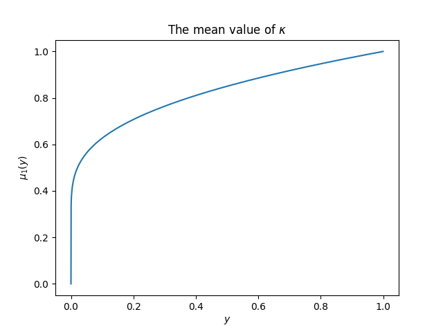
</p>
<hr/>
<p>We are now interested in the limit <span class="katex"><span class="katex-mathml"><math xmlns="http://www.w3.org/1998/Math/MathML"><semantics><mrow><mi>n</mi><mo separator="true">,</mo><mi>k</mi><mo>→</mo><mi mathvariant="normal">∞</mi></mrow><annotation encoding="application/x-tex">n,k\to\infty</annotation></semantics></math></span></span> with <span class="katex"><span class="katex-mathml"><math xmlns="http://www.w3.org/1998/Math/MathML"><semantics><mrow><mi>λ</mi><mo><mi mathvariant="normal">≔</mi></mo><mi>k</mi><mi mathvariant="normal">/</mi><mi>n</mi></mrow><annotation encoding="application/x-tex">\lambda\coloneqq k/n</annotation></semantics></math></span></span> fixed. By Stirling’s approximation, we have <span class="katex-display"><span class="katex"><span class="katex-mathml"><math xmlns="http://www.w3.org/1998/Math/MathML" display="block"><semantics><mrow><msub><mi>P</mi><mrow><mi>n</mi><mo separator="true">,</mo><mi>k</mi></mrow></msub><mo stretchy="false">(</mo><mi>m</mi><mo stretchy="false">)</mo><mo>∼</mo><mrow><mo fence="true">(</mo><mi>n</mi><mo>−</mo><mn>1</mn><mo fence="true">)</mo></mrow><mfrac><mrow><msup><mi>k</mi><mrow><mi>k</mi><mo>+</mo><mn>1</mn><mi mathvariant="normal">/</mi><mn>2</mn></mrow></msup><msup><mrow><mo fence="true">(</mo><mi>n</mi><mo>+</mo><mi>k</mi><mo>−</mo><mi>m</mi><mo>−</mo><mn>2</mn><mo fence="true">)</mo></mrow><mrow><mi>n</mi><mo>+</mo><mi>k</mi><mo>−</mo><mi>m</mi><mo>−</mo><mn>2</mn><mo>+</mo><mn>1</mn><mi mathvariant="normal">/</mi><mn>2</mn></mrow></msup></mrow><mrow><msup><mrow><mo fence="true">(</mo><mi>k</mi><mo>−</mo><mi>m</mi><mo fence="true">)</mo></mrow><mrow><mi>k</mi><mo>−</mo><mi>m</mi><mo>+</mo><mn>1</mn><mi mathvariant="normal">/</mi><mn>2</mn></mrow></msup><msup><mrow><mo fence="true">(</mo><mi>n</mi><mo>+</mo><mi>k</mi><mo>−</mo><mn>1</mn><mo fence="true">)</mo></mrow><mrow><mi>n</mi><mo>+</mo><mi>k</mi><mo>−</mo><mn>1</mn><mo>+</mo><mn>1</mn><mi mathvariant="normal">/</mi><mn>2</mn></mrow></msup></mrow></mfrac><msup><mi mathvariant="normal">e</mi><mrow><mi>k</mi><mo>−</mo><mi>m</mi><mo>+</mo><mi>n</mi><mo>+</mo><mi>k</mi><mo>−</mo><mn>1</mn><mo>−</mo><mi>k</mi><mo>−</mo><mi>n</mi><mo>−</mo><mi>k</mi><mo>+</mo><mi>m</mi><mo>+</mo><mn>2</mn></mrow></msup><mi mathvariant="normal">.</mi></mrow><annotation encoding="application/x-tex">P_{n,k}(m)\sim\left(n-1\right)
\frac{k^{k+1/2}\left(n+k-m-2\right)^{n+k-m-2+1/2}}{\left(k-m\right)^{k-m+1/2}\left(n+k-1\right)^{n+k-1+1/2} }
\mathrm e^{k-m+n+k-1-k-n-k+m+2}.</annotation></semantics></math></span></span></span> The <span class="katex"><span class="katex-mathml"><math xmlns="http://www.w3.org/1998/Math/MathML"><semantics><mrow><mn>1</mn><mi mathvariant="normal">/</mi><mn>2</mn></mrow><annotation encoding="application/x-tex">1/2</annotation></semantics></math></span></span>’s in the exponents can just be dropped because you may find that if we extract the <span class="katex"><span class="katex-mathml"><math xmlns="http://www.w3.org/1998/Math/MathML"><semantics><mrow><mn>1</mn><mi mathvariant="normal">/</mi><mn>2</mn></mrow><annotation encoding="application/x-tex">1/2</annotation></semantics></math></span></span>’s, the factor tends to unity. The exponential is just constant <span class="katex"><span class="katex-mathml"><math xmlns="http://www.w3.org/1998/Math/MathML"><semantics><mrow><mi mathvariant="normal">e</mi></mrow><annotation encoding="application/x-tex">\mathrm e</annotation></semantics></math></span></span>. Therefore, we have
<span class="katex-display"><span class="katex"><span class="katex-mathml"><math xmlns="http://www.w3.org/1998/Math/MathML" display="block"><semantics><mtable rowspacing="0.25em" columnalign="right left" columnspacing="0em"><mtr><mtd><mstyle scriptlevel="0" displaystyle="true"><mrow><msub><mi>P</mi><mrow><mi>n</mi><mo separator="true">,</mo><mi>k</mi></mrow></msub><mo stretchy="false">(</mo><mi>m</mi><mo stretchy="false">)</mo></mrow></mstyle></mtd><mtd><mstyle scriptlevel="0" displaystyle="true"><mrow><mrow/><mo>∼</mo><mrow><mo fence="true">(</mo><mi>n</mi><mo>−</mo><mn>1</mn><mo fence="true">)</mo></mrow><mfrac><mrow><msup><mrow><mo fence="true">(</mo><mi>λ</mi><mi>n</mi><mo fence="true">)</mo></mrow><mrow><mi>λ</mi><mi>n</mi></mrow></msup><msup><mrow><mo fence="true">(</mo><mi>n</mi><mo>+</mo><mi>λ</mi><mi>n</mi><mo>−</mo><mi>m</mi><mo>−</mo><mn>2</mn><mo fence="true">)</mo></mrow><mrow><mi>n</mi><mo>+</mo><mi>λ</mi><mi>n</mi><mo>−</mo><mi>m</mi><mo>−</mo><mn>2</mn></mrow></msup></mrow><mrow><msup><mrow><mo fence="true">(</mo><mi>λ</mi><mi>n</mi><mo>−</mo><mi>m</mi><mo fence="true">)</mo></mrow><mrow><mi>λ</mi><mi>n</mi><mo>−</mo><mi>m</mi></mrow></msup><msup><mrow><mo fence="true">(</mo><mi>n</mi><mo>+</mo><mi>λ</mi><mi>n</mi><mo>−</mo><mn>1</mn><mo fence="true">)</mo></mrow><mrow><mi>n</mi><mo>+</mo><mi>λ</mi><mi>n</mi><mo>−</mo><mn>1</mn></mrow></msup></mrow></mfrac><mi mathvariant="normal">e</mi></mrow></mstyle></mtd></mtr><mtr><mtd><mstyle scriptlevel="0" displaystyle="true"><mrow/></mstyle></mtd><mtd><mstyle scriptlevel="0" displaystyle="true"><mrow><mrow/><mo>=</mo><msup><mrow><mo fence="true">(</mo><mstyle displaystyle="false" scriptlevel="0"><mfrac><mrow><mi>n</mi><mo>+</mo><mi>λ</mi><mi>n</mi><mo>−</mo><mi>m</mi><mo>−</mo><mn>2</mn></mrow><mrow><mi>n</mi><mo>+</mo><mi>λ</mi><mi>n</mi><mo>−</mo><mn>1</mn></mrow></mfrac></mstyle><mo fence="true">)</mo></mrow><mi>n</mi></msup><msup><mrow><mo fence="true">(</mo><mstyle displaystyle="false" scriptlevel="0"><mfrac><mrow><mrow><mo fence="true">(</mo><mi>n</mi><mo>+</mo><mi>λ</mi><mi>n</mi><mo>−</mo><mi>m</mi><mo>−</mo><mn>2</mn><mo fence="true">)</mo></mrow><mi>λ</mi><mi>n</mi></mrow><mrow><mrow><mo fence="true">(</mo><mi>λ</mi><mi>n</mi><mo>−</mo><mi>m</mi><mo fence="true">)</mo></mrow><mrow><mo fence="true">(</mo><mi>n</mi><mo>+</mo><mi>λ</mi><mi>n</mi><mo>−</mo><mn>1</mn><mo fence="true">)</mo></mrow></mrow></mfrac></mstyle><mo fence="true">)</mo></mrow><mrow><mi>λ</mi><mi>n</mi></mrow></msup><msup><mrow><mo fence="true">(</mo><mstyle displaystyle="false" scriptlevel="0"><mfrac><mrow><mi>λ</mi><mi>n</mi><mo>−</mo><mi>m</mi></mrow><mrow><mi>n</mi><mo>+</mo><mi>λ</mi><mi>n</mi><mo>−</mo><mi>m</mi><mo>−</mo><mn>2</mn></mrow></mfrac></mstyle><mo fence="true">)</mo></mrow><mi>m</mi></msup><mstyle displaystyle="false" scriptlevel="0"><mfrac><mrow><mrow><mo fence="true">(</mo><mi>n</mi><mo>−</mo><mn>1</mn><mo fence="true">)</mo></mrow><mrow><mo fence="true">(</mo><mi>n</mi><mo>+</mo><mi>λ</mi><mi>n</mi><mo>−</mo><mn>1</mn><mo fence="true">)</mo></mrow></mrow><msup><mrow><mo fence="true">(</mo><mi>n</mi><mo>+</mo><mi>λ</mi><mi>n</mi><mo>−</mo><mi>m</mi><mo>−</mo><mn>2</mn><mo fence="true">)</mo></mrow><mn>2</mn></msup></mfrac></mstyle><mi mathvariant="normal">e</mi></mrow></mstyle></mtd></mtr><mtr><mtd><mstyle scriptlevel="0" displaystyle="true"><mrow/></mstyle></mtd><mtd><mstyle scriptlevel="0" displaystyle="true"><mrow><mrow/><mo>→</mo><msup><mi mathvariant="normal">e</mi><mrow><mo>−</mo><mfrac><mrow><mi>m</mi><mo>+</mo><mn>1</mn></mrow><mrow><mi>λ</mi><mo>+</mo><mn>1</mn></mrow></mfrac></mrow></msup><mtext> </mtext><msup><mi mathvariant="normal">e</mi><mi>m</mi></msup><mtext> </mtext><msup><mi mathvariant="normal">e</mi><mrow><mo>−</mo><mfrac><mrow><mi>m</mi><mo>+</mo><mn>1</mn></mrow><mrow><mi>λ</mi><mo>+</mo><mn>1</mn></mrow></mfrac><mi>λ</mi></mrow></msup><msup><mrow><mo fence="true">(</mo><mstyle displaystyle="false" scriptlevel="0"><mfrac><mi>λ</mi><mrow><mi>λ</mi><mo>+</mo><mn>1</mn></mrow></mfrac></mstyle><mo fence="true">)</mo></mrow><mi>m</mi></msup><mstyle displaystyle="false" scriptlevel="0"><mfrac><mn>1</mn><mrow><mi>λ</mi><mo>+</mo><mn>1</mn></mrow></mfrac></mstyle><mi mathvariant="normal">e</mi></mrow></mstyle></mtd></mtr><mtr><mtd><mstyle scriptlevel="0" displaystyle="true"><mrow/></mstyle></mtd><mtd><mstyle scriptlevel="0" displaystyle="true"><mrow><mrow/><mo>=</mo><msup><mrow><mo fence="true">(</mo><mstyle displaystyle="false" scriptlevel="0"><mfrac><mi>λ</mi><mrow><mi>λ</mi><mo>+</mo><mn>1</mn></mrow></mfrac></mstyle><mo fence="true">)</mo></mrow><mi>m</mi></msup><mstyle displaystyle="false" scriptlevel="0"><mfrac><mn>1</mn><mrow><mi>λ</mi><mo>+</mo><mn>1</mn></mrow></mfrac></mstyle><mi mathvariant="normal">.</mi></mrow></mstyle></mtd></mtr></mtable><annotation encoding="application/x-tex">\begin{align*}
P_{n,k}(m)&amp;\sim\left(n-1\right)
\frac{\left(\lambda n\right)^{\lambda n}\left(n+\lambda n-m-2\right)^{n+\lambda n-m-2} }
{\left(\lambda n-m\right)^{\lambda n-m}\left(n+\lambda n-1\right)^{n+\lambda n-1}}\mathrm e\\
&amp;=\left(\tfrac{n+\lambda n-m-2}{n+\lambda n-1}\right)^n
\left(\tfrac{\left(n+\lambda n-m-2\right)\lambda n}{\left(\lambda n-m\right)\left(n+\lambda n-1\right)}\right)^{\lambda n}
\left(\tfrac{\lambda n-m}{n+\lambda n-m-2}\right)^m
\tfrac{\left(n-1\right)\left(n+\lambda n-1\right)}{\left(n+\lambda n-m-2\right)^2}\mathrm e\\
&amp;\to\mathrm e^{-\frac{m+1}{\lambda+1}}\,\mathrm e^m\,
\mathrm e^{-\frac{m+1}{\lambda+1}\lambda}\left(\tfrac\lambda{\lambda+1}\right)^m\tfrac1{\lambda+1}\mathrm e\\
&amp;=\left(\tfrac\lambda{\lambda+1}\right)^m\tfrac1{\lambda+1}.
\end{align*}</annotation></semantics></math></span></span></span>
This is just the geometric distribution with parameter <span class="katex"><span class="katex-mathml"><math xmlns="http://www.w3.org/1998/Math/MathML"><semantics><mrow><mi>p</mi><mo>=</mo><mn>1</mn><mi mathvariant="normal">/</mi><mo stretchy="false">(</mo><mi>λ</mi><mo>+</mo><mn>1</mn><mo stretchy="false">)</mo><mo>=</mo><mi>n</mi><mi mathvariant="normal">/</mi><mo stretchy="false">(</mo><mi>k</mi><mo>+</mo><mi>n</mi><mo stretchy="false">)</mo></mrow><annotation encoding="application/x-tex">p=1/(\lambda+1)=n/(k+n)</annotation></semantics></math></span></span>.</p>
<hr/>
<p>If you want to simulate the number of balls in a box, here is a simple way to do this. First, because each box is the same, we can just focus on the first box without loss of generality. Then, we just need to randomly generate the positions of the <span class="katex"><span class="katex-mathml"><math xmlns="http://www.w3.org/1998/Math/MathML"><semantics><mrow><mi>n</mi><mo>−</mo><mn>1</mn></mrow><annotation encoding="application/x-tex">n-1</annotation></semantics></math></span></span> bars among the <span class="katex"><span class="katex-mathml"><math xmlns="http://www.w3.org/1998/Math/MathML"><semantics><mrow><mi>n</mi><mo>+</mo><mi>k</mi><mo>−</mo><mn>1</mn></mrow><annotation encoding="application/x-tex">n+k-1</annotation></semantics></math></span></span> positions, and then return the index of the first bar (which is the number of balls in the first box).</p>
<p>We can then write the following Ruby code to simulate the number of balls in the first box:</p>
<table class="rouge-table">
  <tbody>
    <tr>
      <td class="highlight language-ruby">
        <pre>
          <code>
            <span class="line line-1"><span class="k">def</span> <span class="nf">simulate</span> <span class="n">n</span><span class="p">,</span> <span class="n">k</span>
</span>
            <span class="line line-2">  <span class="p">(</span><span class="n">n</span><span class="o">-</span><span class="mi">1</span><span class="p">).</span><span class="nf">times</span><span class="p">.</span><span class="nf">inject</span><span class="p">(</span><span class="n">npkm1</span> <span class="o">=</span> <span class="n">n</span><span class="o">+</span><span class="n">k</span><span class="o">-</span><span class="mi">1</span><span class="p">)</span> <span class="p">{</span> <span class="o">|</span><span class="n">bar</span><span class="p">,</span> <span class="n">i</span><span class="o">|</span> <span class="p">[</span><span class="nb">rand</span><span class="p">(</span><span class="n">npkm1</span> <span class="o">-</span> <span class="n">i</span><span class="p">),</span> <span class="n">bar</span><span class="p">].</span><span class="nf">min</span> <span class="p">}</span>
</span>
            <span class="line line-3"><span class="k">end</span>
</span>
          </code>
        </pre>
      </td>
    </tr>
  </tbody>
</table>
<p>Compare the simulated result with the theoretical result:</p>
<table class="rouge-table">
  <tbody>
    <tr>
      <td class="highlight language-ruby">
        <pre>
          <code>
            <span class="line line-1"><span class="k">def</span> <span class="nf">frequency</span> <span class="n">m</span><span class="p">,</span> <span class="n">n</span><span class="p">,</span> <span class="n">k</span><span class="p">,</span> <span class="n">trials</span>
</span>
            <span class="line line-2">  <span class="n">trials</span><span class="p">.</span><span class="nf">times</span><span class="p">.</span><span class="nf">count</span> <span class="p">{</span> <span class="n">simulate</span><span class="p">(</span><span class="n">n</span><span class="p">,</span> <span class="n">k</span><span class="p">)</span> <span class="o">==</span> <span class="n">m</span> <span class="p">}</span> <span class="o">/</span> <span class="n">trials</span><span class="p">.</span><span class="nf">to_f</span>
</span>
            <span class="line line-3"><span class="k">end</span>
</span>
            <span class="line line-4">
</span>
            <span class="line line-5"><span class="k">def</span> <span class="nf">truth</span> <span class="n">m</span><span class="p">,</span> <span class="n">n</span><span class="p">,</span> <span class="n">k</span>
</span>
            <span class="line line-6">  <span class="p">(</span><span class="n">n</span><span class="o">-</span><span class="mi">1</span><span class="p">)</span> <span class="o">*</span> <span class="p">(</span><span class="n">k</span><span class="o">-</span><span class="n">m</span><span class="o">+</span><span class="mi">1</span><span class="o">..</span><span class="n">k</span><span class="p">).</span><span class="nf">reduce</span><span class="p">(</span><span class="mi">1</span><span class="p">,:</span><span class="o">*</span><span class="p">)</span> <span class="o">/</span> <span class="p">(</span><span class="n">n</span><span class="o">+</span><span class="n">k</span><span class="o">-</span><span class="n">m</span><span class="o">-</span><span class="mi">1</span><span class="o">..</span><span class="n">n</span><span class="o">+</span><span class="n">k</span><span class="o">-</span><span class="mi">1</span><span class="p">).</span><span class="nf">reduce</span><span class="p">(</span><span class="mi">1</span><span class="p">,:</span><span class="o">*</span><span class="p">).</span><span class="nf">to_f</span>
</span>
            <span class="line line-7"><span class="k">end</span>
</span>
            <span class="line line-8">
</span>
            <span class="line line-9"><span class="k">def</span> <span class="nf">approx</span> <span class="n">m</span><span class="p">,</span> <span class="n">n</span><span class="p">,</span> <span class="n">k</span>
</span>
            <span class="line line-10">  <span class="n">n</span><span class="o">*</span><span class="n">k</span><span class="o">**</span><span class="n">m</span> <span class="o">/</span> <span class="p">((</span><span class="n">n</span><span class="o">+</span><span class="n">k</span><span class="p">)</span><span class="o">**</span><span class="p">(</span><span class="n">m</span><span class="o">+</span><span class="mi">1</span><span class="p">)).</span><span class="nf">to_f</span>
</span>
            <span class="line line-11"><span class="k">end</span>
</span>
            <span class="line line-12">
</span>
            <span class="line line-13"><span class="nb">srand</span> <span class="mi">1108</span>
</span>
            <span class="line line-14"><span class="n">m</span><span class="p">,</span> <span class="n">n</span><span class="p">,</span> <span class="n">k</span> <span class="o">=</span> <span class="mi">3</span><span class="p">,</span> <span class="mi">5000</span><span class="p">,</span> <span class="mi">8000</span>
</span>
            <span class="line line-15"><span class="nb">p</span> <span class="n">frequency</span> <span class="n">m</span><span class="p">,</span> <span class="n">n</span><span class="p">,</span> <span class="n">k</span><span class="p">,</span> <span class="mi">10000</span> <span class="c1"># =&gt; 0.0902</span>
</span>
            <span class="line line-16"><span class="nb">p</span> <span class="n">truth</span> <span class="n">m</span><span class="p">,</span> <span class="n">n</span><span class="p">,</span> <span class="n">k</span> <span class="c1"># =&gt; 0.08965012972626446</span>
</span>
            <span class="line line-17"><span class="nb">p</span> <span class="n">approx</span> <span class="n">m</span><span class="p">,</span> <span class="n">n</span><span class="p">,</span> <span class="n">k</span> <span class="c1"># =&gt; 0.08963271594131858</span>
</span>
          </code>
        </pre>
      </td>
    </tr>
  </tbody>
</table>]]></content><author><name>UlyssesZhan</name><email>ulysseszhan@gmail.com</email></author><category term="math" /><category term="probability" /><category term="combinatorics" /><category term="ruby" /><summary type="html"><![CDATA[Suppose there are <span class="katex"><span class="katex-mathml"><math xmlns="http://www.w3.org/1998/Math/MathML"><semantics><mrow><mi>n</mi></mrow><annotation encoding="application/x-tex">n</annotation></semantics></math></span></span> distinguishable boxes and <span class="katex"><span class="katex-mathml"><math xmlns="http://www.w3.org/1998/Math/MathML"><semantics><mrow><mi>k</mi></mrow><annotation encoding="application/x-tex">k</annotation></semantics></math></span></span> indistinguishable balls. Now, we randomly put the balls into the boxes. For each of the boxes, what is the probability that it contains <span class="katex"><span class="katex-mathml"><math xmlns="http://www.w3.org/1998/Math/MathML"><semantics><mrow><mi>m</mi></mrow><annotation encoding="application/x-tex">m</annotation></semantics></math></span></span> balls? This is a simple combanitorics problem that can be solved by the stars and bars method. It turns out that in the limit <span class="katex"><span class="katex-mathml"><math xmlns="http://www.w3.org/1998/Math/MathML"><semantics><mrow><mi>n</mi><mo separator="true">,</mo><mi>k</mi><mo>→</mo><mi mathvariant="normal">∞</mi></mrow><annotation encoding="application/x-tex">n,k\to\infty</annotation></semantics></math></span></span> with <span class="katex"><span class="katex-mathml"><math xmlns="http://www.w3.org/1998/Math/MathML"><semantics><mrow><mi>k</mi><mi mathvariant="normal">/</mi><mi>n</mi></mrow><annotation encoding="application/x-tex">k/n</annotation></semantics></math></span></span> fixed, the distribution tends to be a geometric distribution.]]></summary><media:thumbnail xmlns:media="http://search.yahoo.com/mrss/" url="https://ulysseszh.github.io/assets/images/covers/2023-05-09-stars-bars-geometric.png" /><media:content medium="image" url="https://ulysseszh.github.io/assets/images/covers/2023-05-09-stars-bars-geometric.png" xmlns:media="http://search.yahoo.com/mrss/" /></entry><entry><title type="html"><![CDATA[Introducing bra–ket notation to math learners]]></title><link href="https://ulysseszh.github.io/math/2023/02/03/math-braket.html" rel="alternate" type="text/html" title="Introducing bra–ket notation to math learners" /><published>2023-02-03T15:12:53-08:00</published><updated>2023-02-03T15:12:53-08:00</updated><id>https://ulysseszh.github.io/math/2023/02/03/math-braket</id><content type="html" xml:base="https://ulysseszh.github.io/math/2023/02/03/math-braket.html"><![CDATA[<p>
  <em>This article is translated from a Chinese <a href="https://zhuanlan.zhihu.com/p/344660674" target="_blank" rel="external">article</a> on my Zhihu account. The original article was posted at 2021-01-16 15:52 +0800.</em>
</p>
<hr/>
<p>To keep you guys that have read different textbooks from fighting with each other, we say:</p>
<ul>
<li>The definition of inner products is opposite in math and physics, and we take the customary definition in math as the standard: inner products are linear in the first element and conjugate-linear in the second element.</li>
<li>Denote Hilbert space by <span class="katex"><span class="katex-mathml"><math xmlns="http://www.w3.org/1998/Math/MathML"><semantics><mrow><mi mathvariant="script">H</mi></mrow><annotation encoding="application/x-tex">\mathscr H</annotation></semantics></math></span></span>. Denote inner products by <span class="katex"><span class="katex-mathml"><math xmlns="http://www.w3.org/1998/Math/MathML"><semantics><mrow><mo fence="true">(</mo><mo>⋅</mo><mo separator="true">,</mo><mo>⋅</mo><mo fence="true">)</mo></mrow><annotation encoding="application/x-tex">\left(\cdot,\cdot\right)</annotation></semantics></math></span></span>.</li>
<li>Denote the dual space of <span class="katex"><span class="katex-mathml"><math xmlns="http://www.w3.org/1998/Math/MathML"><semantics><mrow><mi>V</mi></mrow><annotation encoding="application/x-tex">V</annotation></semantics></math></span></span> as <span class="katex"><span class="katex-mathml"><math xmlns="http://www.w3.org/1998/Math/MathML"><semantics><mrow><msup><mi>V</mi><mo>∗</mo></msup></mrow><annotation encoding="application/x-tex">V^*</annotation></semantics></math></span></span>. Denote the Hermite adjoint of <span class="katex"><span class="katex-mathml"><math xmlns="http://www.w3.org/1998/Math/MathML"><semantics><mrow><mover accent="true"><mi>T</mi><mo>^</mo></mover></mrow><annotation encoding="application/x-tex">\hat T</annotation></semantics></math></span></span> as <span class="katex"><span class="katex-mathml"><math xmlns="http://www.w3.org/1998/Math/MathML"><semantics><mrow><msup><mover accent="true"><mi>T</mi><mo>^</mo></mover><mo>†</mo></msup></mrow><annotation encoding="application/x-tex">\hat T^\dagger</annotation></semantics></math></span></span>. Denote the complex conjugate of <span class="katex"><span class="katex-mathml"><math xmlns="http://www.w3.org/1998/Math/MathML"><semantics><mrow><mi>α</mi></mrow><annotation encoding="application/x-tex">\alpha</annotation></semantics></math></span></span> as <span class="katex"><span class="katex-mathml"><math xmlns="http://www.w3.org/1998/Math/MathML"><semantics><mrow><mover accent="true"><mi>α</mi><mo>ˉ</mo></mover></mrow><annotation encoding="application/x-tex">\bar\alpha</annotation></semantics></math></span></span>.</li>
<li>Denote the set of all bounded linear operators in <span class="katex"><span class="katex-mathml"><math xmlns="http://www.w3.org/1998/Math/MathML"><semantics><mrow><mi>V</mi><mo>→</mo><mi>V</mi></mrow><annotation encoding="application/x-tex">V\to V</annotation></semantics></math></span></span> as <span class="katex"><span class="katex-mathml"><math xmlns="http://www.w3.org/1998/Math/MathML"><semantics><mrow><mi mathvariant="script">L</mi><mo stretchy="false">(</mo><mi>V</mi><mo stretchy="false">)</mo></mrow><annotation encoding="application/x-tex">\mathcal L(V)</annotation></semantics></math></span></span>.</li>
</ul>
<hr/>
<p>Riesz representation theorem points out that <span class="katex-display"><span class="katex"><span class="katex-mathml"><math xmlns="http://www.w3.org/1998/Math/MathML" display="block"><semantics><mrow><mi mathvariant="normal">∀</mi><mrow><mo fence="true">&lt;</mo><mi>z</mi><mo fence="true">∣</mo></mrow><mo>∈</mo><msup><mi mathvariant="script">H</mi><mo>∗</mo></msup><mo>:</mo><mi mathvariant="normal">∃</mi><mo stretchy="false">!</mo><mrow><mo fence="true">∣</mo><mi>z</mi><mo fence="true">&gt;</mo></mrow><mo>∈</mo><mi mathvariant="script">H</mi><mo>:</mo><mi mathvariant="normal">∀</mi><mrow><mo fence="true">∣</mo><mi>x</mi><mo fence="true">&gt;</mo></mrow><mo>∈</mo><mi mathvariant="script">H</mi><mo>:</mo><mrow><mo fence="true">&lt;</mo><mi>z</mi><mo fence="true" lspace="0.05em" rspace="0.05em">|</mo><mi>x</mi><mo fence="true">&gt;</mo></mrow><mo>=</mo><mrow><mo fence="true">(</mo><mrow><mo fence="true">∣</mo><mi>x</mi><mo fence="true">&gt;</mo></mrow><mo separator="true">,</mo><mrow><mo fence="true">∣</mo><mi>z</mi><mo fence="true">&gt;</mo></mrow><mo fence="true">)</mo></mrow><mo separator="true">,</mo></mrow><annotation encoding="application/x-tex">\forall \left&lt;z\right|\in\mathscr H^*:
\exists!\left|z\right&gt;\in\mathscr H:
\forall\left|x\right&gt;\in\mathscr H:
\left&lt;z\middle|x\right&gt;=\left(\left|x\right&gt;,\left|z\right&gt;\right),</annotation></semantics></math></span></span></span> which naturally gives a norm-preserving anti-isomorphism of <span class="katex"><span class="katex-mathml"><math xmlns="http://www.w3.org/1998/Math/MathML"><semantics><mrow><msup><mi mathvariant="script">H</mi><mo>∗</mo></msup><mo>→</mo><mi mathvariant="script">H</mi></mrow><annotation encoding="application/x-tex">\mathscr H^*\to\mathscr H</annotation></semantics></math></span></span> given by <span class="katex"><span class="katex-mathml"><math xmlns="http://www.w3.org/1998/Math/MathML"><semantics><mrow><mrow><mo fence="true">&lt;</mo><mi>z</mi><mo fence="true">∣</mo></mrow><mo>↦</mo><mrow><mo fence="true">∣</mo><mi>z</mi><mo fence="true">&gt;</mo></mrow></mrow><annotation encoding="application/x-tex">\left&lt;z\right|\mapsto\left|z\right&gt;</annotation></semantics></math></span></span>.</p>
<p>(Actually, furthermore, we can study rigged Hilbert spaces, but it is more complex in terms of mathematics, and we currently only look at Hilbert spaces.)</p>
<p>
  <strong>Now, bra–ket notation shows its first good-looking feature: use <span class="katex"><span class="katex-mathml"><math xmlns="http://www.w3.org/1998/Math/MathML"><semantics><mrow><mo fence="true">&lt;</mo><mo>⋅</mo><mo fence="true" lspace="0.05em" rspace="0.05em">|</mo><mo>⋅</mo><mo fence="true">&gt;</mo></mrow><annotation encoding="application/x-tex">\left&lt;\cdot\middle|\cdot\right&gt;</annotation></semantics></math></span></span> to represent inner products.</strong>
</p>
<p>To generalize inner products, we define sesquilinear forms on <span class="katex"><span class="katex-mathml"><math xmlns="http://www.w3.org/1998/Math/MathML"><semantics><mrow><mi mathvariant="script">H</mi></mrow><annotation encoding="application/x-tex">\mathscr H</annotation></semantics></math></span></span> as mappings of <span class="katex"><span class="katex-mathml"><math xmlns="http://www.w3.org/1998/Math/MathML"><semantics><mrow><mi mathvariant="script">H</mi><mo>×</mo><mi mathvariant="script">H</mi><mo>→</mo><mi mathvariant="double-struck">C</mi></mrow><annotation encoding="application/x-tex">\mathscr H\times\mathscr H\to\mathbb C</annotation></semantics></math></span></span>, which is linear in the first element and conjugate-linear in the second element.</p>
<p>We can prove that, for a sequilinear form <span class="katex"><span class="katex-mathml"><math xmlns="http://www.w3.org/1998/Math/MathML"><semantics><mrow><mi>φ</mi></mrow><annotation encoding="application/x-tex">\varphi</annotation></semantics></math></span></span>, if <span class="katex-display"><span class="katex"><span class="katex-mathml"><math xmlns="http://www.w3.org/1998/Math/MathML" display="block"><semantics><mrow><mi mathvariant="normal">∃</mi><mi>C</mi><mo>&gt;</mo><mn>0</mn><mo>:</mo><mi mathvariant="normal">∀</mi><mrow><mo fence="true">∣</mo><mi>x</mi><mo fence="true">&gt;</mo></mrow><mo separator="true">,</mo><mrow><mo fence="true">∣</mo><mi>y</mi><mo fence="true">&gt;</mo></mrow><mo>∈</mo><mi mathvariant="script">H</mi><mo>:</mo><msup><mrow><mo fence="true">∣</mo><mi>φ</mi><mtext> ⁣</mtext><mrow><mo fence="true">(</mo><mrow><mo fence="true">∣</mo><mi>x</mi><mo fence="true">&gt;</mo></mrow><mo separator="true">,</mo><mrow><mo fence="true">∣</mo><mi>y</mi><mo fence="true">&gt;</mo></mrow><mo fence="true">)</mo></mrow><mo fence="true">∣</mo></mrow><mn>2</mn></msup><mo>≤</mo><mi>C</mi><mrow><mo fence="true">&lt;</mo><mi>x</mi><mo fence="true" lspace="0.05em" rspace="0.05em">|</mo><mi>x</mi><mo fence="true">&gt;</mo></mrow><mrow><mo fence="true">&lt;</mo><mi>y</mi><mo fence="true" lspace="0.05em" rspace="0.05em">|</mo><mi>y</mi><mo fence="true">&gt;</mo></mrow></mrow><annotation encoding="application/x-tex">\exists C&gt;0:
\forall\left|x\right&gt;,\left|y\right&gt;\in\mathscr H:
\left|\varphi\!\left(\left|x\right&gt;,\left|y\right&gt;\right)\right|^2\le C\left&lt;x\middle|x\right&gt;\left&lt;y\middle|y\right&gt;</annotation></semantics></math></span></span></span> (i.e. <span class="katex"><span class="katex-mathml"><math xmlns="http://www.w3.org/1998/Math/MathML"><semantics><mrow><mi>φ</mi></mrow><annotation encoding="application/x-tex">\varphi</annotation></semantics></math></span></span> is bounded), then there exists unique <span class="katex"><span class="katex-mathml"><math xmlns="http://www.w3.org/1998/Math/MathML"><semantics><mrow><mover accent="true"><mi>a</mi><mo>^</mo></mover><mo>∈</mo><mi mathvariant="script">L</mi><mo stretchy="false">(</mo><mi mathvariant="script">H</mi><mo stretchy="false">)</mo></mrow><annotation encoding="application/x-tex">\hat a\in\mathcal L(\mathscr H)</annotation></semantics></math></span></span> such that <span class="katex-display"><span class="katex"><span class="katex-mathml"><math xmlns="http://www.w3.org/1998/Math/MathML" display="block"><semantics><mrow><mi mathvariant="normal">∀</mi><mrow><mo fence="true">∣</mo><mi>x</mi><mo fence="true">&gt;</mo></mrow><mo separator="true">,</mo><mrow><mo fence="true">∣</mo><mi>y</mi><mo fence="true">&gt;</mo></mrow><mo>∈</mo><mi mathvariant="script">H</mi><mo>:</mo><mrow><mo fence="true">&lt;</mo><mi>x</mi><mo fence="true" lspace="0.05em" rspace="0.05em">|</mo><msup><mover accent="true"><mi>a</mi><mo>^</mo></mover><mo>†</mo></msup><mo fence="true" lspace="0.05em" rspace="0.05em">|</mo><mi>y</mi><mo fence="true">&gt;</mo></mrow><mo>=</mo><mover accent="true"><mrow><mo fence="true">&lt;</mo><mi>y</mi><mo fence="true" lspace="0.05em" rspace="0.05em">|</mo><mover accent="true"><mi>a</mi><mo>^</mo></mover><mo fence="true" lspace="0.05em" rspace="0.05em">|</mo><mi>x</mi><mo fence="true">&gt;</mo></mrow><mo stretchy="true">‾</mo></mover><mo separator="true">,</mo></mrow><annotation encoding="application/x-tex">\forall\left|x\right&gt;,\left|y\right&gt;\in\mathscr H:
\left&lt;x\middle|\hat a^\dagger\middle|y\right&gt;=\overline{\left&lt;y\middle|\hat a\middle|x\right&gt;},</annotation></semantics></math></span></span></span> which is rather good-looking.</p>
<p>
  <strong>Now, bra–ket notation shows its second good-looking feature: use <span class="katex"><span class="katex-mathml"><math xmlns="http://www.w3.org/1998/Math/MathML"><semantics><mrow><mo fence="true">&lt;</mo><mo>⋅</mo><mo fence="true" lspace="0.05em" rspace="0.05em">|</mo><mo>⋅</mo><mo fence="true" lspace="0.05em" rspace="0.05em">|</mo><mo>⋅</mo><mo fence="true">&gt;</mo></mrow><annotation encoding="application/x-tex">\left&lt;\cdot\middle|\cdot\middle|\cdot\right&gt;</annotation></semantics></math></span></span> to represent bounded sesquilinear forms.</strong>
</p>
<p>Obviously, if a countable set <span class="katex"><span class="katex-mathml"><math xmlns="http://www.w3.org/1998/Math/MathML"><semantics><mrow><mo fence="true">{</mo><mrow><mo fence="true">∣</mo><msub><mi>e</mi><mi>n</mi></msub><mo fence="true">&gt;</mo></mrow><mo fence="true">}</mo></mrow><annotation encoding="application/x-tex">\left\{\left|e_n\right&gt;\right\}</annotation></semantics></math></span></span> is an orthonormal basis of <span class="katex"><span class="katex-mathml"><math xmlns="http://www.w3.org/1998/Math/MathML"><semantics><mrow><mi mathvariant="script">H</mi></mrow><annotation encoding="application/x-tex">\mathscr H</annotation></semantics></math></span></span> (countability requires <span class="katex"><span class="katex-mathml"><math xmlns="http://www.w3.org/1998/Math/MathML"><semantics><mrow><mi mathvariant="script">H</mi></mrow><annotation encoding="application/x-tex">\mathscr H</annotation></semantics></math></span></span> to be separable), then <span class="katex-display"><span class="katex"><span class="katex-mathml"><math xmlns="http://www.w3.org/1998/Math/MathML" display="block"><semantics><mrow><munder><mo>∑</mo><mi>n</mi></munder><mrow><mo fence="true">∣</mo><msub><mi>e</mi><mi>n</mi></msub><mo fence="true">&gt;</mo></mrow><mrow><mo fence="true">&lt;</mo><msub><mi>e</mi><mi>n</mi></msub><mo fence="true">∣</mo></mrow><mo>=</mo><mrow><mi mathvariant="normal">i</mi><mi mathvariant="normal">d</mi></mrow><mi mathvariant="normal">.</mi></mrow><annotation encoding="application/x-tex">\sum_n\left|e_n\right&gt;\left&lt;e_n\right|=\mathrm{id}.</annotation></semantics></math></span></span></span> Such way of expressing completeness is very good-looking.</p>
<p>If <span class="katex"><span class="katex-mathml"><math xmlns="http://www.w3.org/1998/Math/MathML"><semantics><mrow><mover accent="true"><mi>a</mi><mo>^</mo></mover><mo>∈</mo><mi mathvariant="script">L</mi><mo stretchy="false">(</mo><mi mathvariant="script">H</mi><mo stretchy="false">)</mo></mrow><annotation encoding="application/x-tex">\hat a\in\mathcal L(\mathscr H)</annotation></semantics></math></span></span> has set of eigenvectors <span class="katex"><span class="katex-mathml"><math xmlns="http://www.w3.org/1998/Math/MathML"><semantics><mrow><mo fence="true">{</mo><mrow><mo fence="true">∣</mo><msub><mi>e</mi><mi>n</mi></msub><mo fence="true">&gt;</mo></mrow><mo fence="true">}</mo></mrow><annotation encoding="application/x-tex">\left\{\left|e_n\right&gt;\right\}</annotation></semantics></math></span></span> (already orthonormalized and countable) is complete, then we have the spectral decomposition <span class="katex-display"><span class="katex"><span class="katex-mathml"><math xmlns="http://www.w3.org/1998/Math/MathML" display="block"><semantics><mrow><mover accent="true"><mi>a</mi><mo>^</mo></mover><mo>=</mo><munder><mo>∑</mo><mi>n</mi></munder><msub><mi>a</mi><mi>n</mi></msub><mrow><mo fence="true">∣</mo><msub><mi>e</mi><mi>n</mi></msub><mo fence="true">&gt;</mo></mrow><mo separator="true">,</mo></mrow><annotation encoding="application/x-tex">\hat a=\sum_na_n\left|e_n\right&gt;,</annotation></semantics></math></span></span></span> where <span class="katex"><span class="katex-mathml"><math xmlns="http://www.w3.org/1998/Math/MathML"><semantics><mrow><mo fence="true">{</mo><msub><mi>a</mi><mi>n</mi></msub><mo fence="true">}</mo></mrow><annotation encoding="application/x-tex">\left\{a_n\right\}</annotation></semantics></math></span></span> is the point spectrum of <span class="katex"><span class="katex-mathml"><math xmlns="http://www.w3.org/1998/Math/MathML"><semantics><mrow><mover accent="true"><mi>a</mi><mo>^</mo></mover></mrow><annotation encoding="application/x-tex">\hat a</annotation></semantics></math></span></span>:
<span class="katex-display"><span class="katex"><span class="katex-mathml"><math xmlns="http://www.w3.org/1998/Math/MathML" display="block"><semantics><mrow><mover accent="true"><mi>a</mi><mo>^</mo></mover><mrow><mo fence="true">∣</mo><msub><mi>e</mi><mi>n</mi></msub><mo fence="true">&gt;</mo></mrow><mo>=</mo><msub><mi>a</mi><mi>n</mi></msub><mrow><mo fence="true">∣</mo><msub><mi>e</mi><mi>n</mi></msub><mo fence="true">&gt;</mo></mrow><mi mathvariant="normal">.</mi></mrow><annotation encoding="application/x-tex">\hat a\left|e_n\right&gt;=a_n\left|e_n\right&gt;.</annotation></semantics></math></span></span></span> No wonder why physicists like bra–ket notation. After all, to write <span class="katex-display"><span class="katex"><span class="katex-mathml"><math xmlns="http://www.w3.org/1998/Math/MathML" display="block"><semantics><mrow><mi mathvariant="normal">Pr</mi><mo>⁡</mo><mtext> ⁣</mtext><mrow><mo fence="true">(</mo><mi>a</mi><mo>=</mo><msub><mi>a</mi><mi>n</mi></msub><mo fence="true">)</mo></mrow><mo>=</mo><msup><mrow><mo fence="true">∣</mo><mrow><mo fence="true">&lt;</mo><msub><mi>e</mi><mi>n</mi></msub><mo fence="true" lspace="0.05em" rspace="0.05em">|</mo><mi>ψ</mi><mo fence="true">&gt;</mo></mrow><mo fence="true">∣</mo></mrow><mn>2</mn></msup></mrow><annotation encoding="application/x-tex">\operatorname{Pr}\!\left(a=a_n\right)=\left|\left&lt;e_n\middle|\psi\right&gt;\right|^2</annotation></semantics></math></span></span></span> (the probability of getting a result of <span class="katex"><span class="katex-mathml"><math xmlns="http://www.w3.org/1998/Math/MathML"><semantics><mrow><msub><mi>a</mi><mi>n</mi></msub></mrow><annotation encoding="application/x-tex">a_n</annotation></semantics></math></span></span> when measuring the observable <span class="katex"><span class="katex-mathml"><math xmlns="http://www.w3.org/1998/Math/MathML"><semantics><mrow><mi>a</mi></mrow><annotation encoding="application/x-tex">a</annotation></semantics></math></span></span> corrresponding to the self-adjoint operator <span class="katex"><span class="katex-mathml"><math xmlns="http://www.w3.org/1998/Math/MathML"><semantics><mrow><mover accent="true"><mi>a</mi><mo>^</mo></mover></mrow><annotation encoding="application/x-tex">\hat a</annotation></semantics></math></span></span> with complete set of eigenvectors) and
<span class="katex-display"><span class="katex"><span class="katex-mathml"><math xmlns="http://www.w3.org/1998/Math/MathML" display="block"><semantics><mrow><mi mathvariant="normal">E</mi><mo>⁡</mo><mtext> ⁣</mtext><mrow><mo fence="true">[</mo><mi>a</mi><mo fence="true">]</mo></mrow><mo>=</mo><mrow><mo fence="true">&lt;</mo><mi>ψ</mi><mo fence="true" lspace="0.05em" rspace="0.05em">|</mo><mover accent="true"><mi>a</mi><mo>^</mo></mover><mo fence="true" lspace="0.05em" rspace="0.05em">|</mo><mi>ψ</mi><mo fence="true">&gt;</mo></mrow></mrow><annotation encoding="application/x-tex">\operatorname{E}\!\left[a\right]=\left&lt;\psi\middle|\hat a\middle|\psi\right&gt;</annotation></semantics></math></span></span></span> (the expectation of <span class="katex"><span class="katex-mathml"><math xmlns="http://www.w3.org/1998/Math/MathML"><semantics><mrow><mi>a</mi></mrow><annotation encoding="application/x-tex">a</annotation></semantics></math></span></span>) is pleasant (<span class="katex"><span class="katex-mathml"><math xmlns="http://www.w3.org/1998/Math/MathML"><semantics><mrow><mo fence="true">∣</mo><mi>ψ</mi><mo fence="true">&gt;</mo></mrow><annotation encoding="application/x-tex">\left|\psi\right&gt;</annotation></semantics></math></span></span> is already normalized).</p>
<hr/>
<p>For sure, there are many more pleasant things out there. It is also happy to write the operator into the argument of the exponential function (because it is like making a very complicated thing look like a very simple thing).</p>
<p>If we assume that the Hamiltonian operator <span class="katex"><span class="katex-mathml"><math xmlns="http://www.w3.org/1998/Math/MathML"><semantics><mrow><mover accent="true"><mi>H</mi><mo>^</mo></mover></mrow><annotation encoding="application/x-tex">\hat H</annotation></semantics></math></span></span> is a bounded linear operator, then <span class="katex"><span class="katex-mathml"><math xmlns="http://www.w3.org/1998/Math/MathML"><semantics><mrow><mo>−</mo><mi mathvariant="normal">i</mi><mover accent="true"><mi>H</mi><mo>^</mo></mover></mrow><annotation encoding="application/x-tex">-\mathrm i\hat H</annotation></semantics></math></span></span> naturally fits the Lipschitz condition, so the Schrödinger equation <span class="katex-display"><span class="katex"><span class="katex-mathml"><math xmlns="http://www.w3.org/1998/Math/MathML" display="block"><semantics><mrow><mfrac><mi mathvariant="normal">d</mi><mrow><mi mathvariant="normal">d</mi><mi>t</mi></mrow></mfrac><mrow><mo fence="true">∣</mo><mi>ψ</mi><mo fence="true">&gt;</mo></mrow><mo>=</mo><mo>−</mo><mi mathvariant="normal">i</mi><mover accent="true"><mi>H</mi><mo>^</mo></mover><mrow><mo fence="true">∣</mo><mi>ψ</mi><mo fence="true">&gt;</mo></mrow></mrow><annotation encoding="application/x-tex">\frac{\mathrm d}{\mathrm dt}\left|\psi\right&gt;=-\mathrm i\hat H\left|\psi\right&gt;</annotation></semantics></math></span></span></span> has a unique solution. Furthermore, if <span class="katex"><span class="katex-mathml"><math xmlns="http://www.w3.org/1998/Math/MathML"><semantics><mrow><mover accent="true"><mi>H</mi><mo>^</mo></mover></mrow><annotation encoding="application/x-tex">\hat H</annotation></semantics></math></span></span> does not depend on <span class="katex"><span class="katex-mathml"><math xmlns="http://www.w3.org/1998/Math/MathML"><semantics><mrow><mi>t</mi></mrow><annotation encoding="application/x-tex">t</annotation></semantics></math></span></span> explicitly, then the solution is <span class="katex-display"><span class="katex"><span class="katex-mathml"><math xmlns="http://www.w3.org/1998/Math/MathML" display="block"><semantics><mrow><mrow><mo fence="true">∣</mo><mi>ψ</mi><mo fence="true">&gt;</mo></mrow><mo>=</mo><msup><mi mathvariant="normal">e</mi><mrow><mo>−</mo><mi mathvariant="normal">i</mi><mi>t</mi><mover accent="true"><mi>H</mi><mo>^</mo></mover></mrow></msup><mrow><mo fence="true">∣</mo><msub><mi>ψ</mi><mn>0</mn></msub><mo fence="true">&gt;</mo></mrow><mi mathvariant="normal">.</mi></mrow><annotation encoding="application/x-tex">\left|\psi\right&gt;=\mathrm e^{-\mathrm it\hat H}\left|\psi_0\right&gt;.</annotation></semantics></math></span></span></span> What is pleasant about writing in this form is (1) that the form is very simple, (2) that it naturally motivates us to find energy eigenstates, and (3) that it naturally makes us find that time evolution is unitary.</p>
<p>(You guys may notice that I ate the reduced Planck constant. Yes, it is so happy to use natural units.)</p>]]></content><author><name>UlyssesZhan</name><email>ulysseszhan@gmail.com</email></author><category term="math" /><category term="from zhihu" /><category term="quantum mechanics" /><summary type="html"><![CDATA[Bra–ket notation is a good-looking notation! I am sad that it is not generally taught in math courses. Let me introduce it to you.]]></summary><media:thumbnail xmlns:media="http://search.yahoo.com/mrss/" url="https://ulysseszh.github.io/assets/images/covers/2023-02-03-math-braket.png" /><media:content medium="image" url="https://ulysseszh.github.io/assets/images/covers/2023-02-03-math-braket.png" xmlns:media="http://search.yahoo.com/mrss/" /></entry><entry><title type="html"><![CDATA[This is what will happen after you get a haircut]]></title><link href="https://ulysseszh.github.io/math/2023/01/18/hair-growth.html" rel="alternate" type="text/html" title="This is what will happen after you get a haircut" /><published>2023-01-18T12:11:41-08:00</published><updated>2023-01-18T12:11:41-08:00</updated><id>https://ulysseszh.github.io/math/2023/01/18/hair-growth</id><content type="html" xml:base="https://ulysseszh.github.io/math/2023/01/18/hair-growth.html"><![CDATA[<p>Denote the length distribution of one’s hair to be <span class="katex"><span class="katex-mathml"><math xmlns="http://www.w3.org/1998/Math/MathML"><semantics><mrow><mi>f</mi><mo stretchy="false">(</mo><mi>l</mi><mo separator="true">,</mo><mi>t</mi><mo stretchy="false">)</mo></mrow><annotation encoding="application/x-tex">f(l,t)</annotation></semantics></math></span></span>. This means that, at time <span class="katex"><span class="katex-mathml"><math xmlns="http://www.w3.org/1998/Math/MathML"><semantics><mrow><mi>t</mi></mrow><annotation encoding="application/x-tex">t</annotation></semantics></math></span></span>, the number of hairs within the length range from <span class="katex"><span class="katex-mathml"><math xmlns="http://www.w3.org/1998/Math/MathML"><semantics><mrow><mi>l</mi></mrow><annotation encoding="application/x-tex">l</annotation></semantics></math></span></span> to <span class="katex"><span class="katex-mathml"><math xmlns="http://www.w3.org/1998/Math/MathML"><semantics><mrow><mi>l</mi><mo>+</mo><mi mathvariant="normal">d</mi><mi>l</mi></mrow><annotation encoding="application/x-tex">l+\mathrm dl</annotation></semantics></math></span></span> is <span class="katex"><span class="katex-mathml"><math xmlns="http://www.w3.org/1998/Math/MathML"><semantics><mrow><mi>N</mi><mi>f</mi><mtext> ⁣</mtext><mrow><mo fence="true">(</mo><mi>l</mi><mo separator="true">,</mo><mi>t</mi><mo fence="true">)</mo></mrow><mi mathvariant="normal">d</mi><mi>l</mi></mrow><annotation encoding="application/x-tex">Nf\!\left(l,t\right)\mathrm dl</annotation></semantics></math></span></span>, where <span class="katex"><span class="katex-mathml"><math xmlns="http://www.w3.org/1998/Math/MathML"><semantics><mrow><mi>N</mi></mrow><annotation encoding="application/x-tex">N</annotation></semantics></math></span></span> is the total number of hairs.</p>
<p>Each hair grows at constant speed <span class="katex"><span class="katex-mathml"><math xmlns="http://www.w3.org/1998/Math/MathML"><semantics><mrow><mi>v</mi></mrow><annotation encoding="application/x-tex">v</annotation></semantics></math></span></span>. However, they cannot grow indefinitely because there is a probability of <span class="katex"><span class="katex-mathml"><math xmlns="http://www.w3.org/1998/Math/MathML"><semantics><mrow><mi>λ</mi></mrow><annotation encoding="application/x-tex">\lambda</annotation></semantics></math></span></span> per unit time for a hair to be lost naturally (this is the same assumption as the exponential decay). After a hair is lost, it restarts growing from zero length.</p>
<p>Suppose that at <span class="katex"><span class="katex-mathml"><math xmlns="http://www.w3.org/1998/Math/MathML"><semantics><mrow><mi>t</mi><mo>=</mo><mn>0</mn></mrow><annotation encoding="application/x-tex">t=0</annotation></semantics></math></span></span> you have got a haircut so that the hair length distribution becomes <span id="eq:eq-initial-condition" data-label="(1)"><span class="katex-display-table"> <span class="katex-display-numbered"><span class="katex-display"><span class="katex"><span class="katex-mathml"><math xmlns="http://www.w3.org/1998/Math/MathML" display="block"><semantics><mrow><mi>f</mi><mo stretchy="false">(</mo><mi>l</mi><mo separator="true">,</mo><mn>0</mn><mo stretchy="false">)</mo><mo>=</mo><msub><mi>f</mi><mn>0</mn></msub><mo stretchy="false">(</mo><mi>l</mi><mo stretchy="false">)</mo><mi mathvariant="normal">.</mi></mrow><annotation encoding="application/x-tex">f(l,0)=f_0(l).</annotation></semantics></math></span></span></span></span> <span class="katex-display-number"><span class="katex-display"><span class="katex"><span class="katex-mathml"><math xmlns="http://www.w3.org/1998/Math/MathML" display="block"><semantics><mrow><mo stretchy="false">(</mo><mn>1</mn><mo stretchy="false">)</mo></mrow><annotation encoding="application/x-tex">(1)</annotation></semantics></math></span></span></span></span> </span></span> Then, how does the distribution evolve with time?</p>
<hr/>
<p>Because <span class="katex"><span class="katex-mathml"><math xmlns="http://www.w3.org/1998/Math/MathML"><semantics><mrow><mi>f</mi></mrow><annotation encoding="application/x-tex">f</annotation></semantics></math></span></span> is a distribution function, There is a normalization restriction on <span class="katex"><span class="katex-mathml"><math xmlns="http://www.w3.org/1998/Math/MathML"><semantics><mrow><mi>f</mi></mrow><annotation encoding="application/x-tex">f</annotation></semantics></math></span></span>: <span id="eq:eq-normalization" data-label="(2)"><span class="katex-display-table"> <span class="katex-display-numbered"><span class="katex-display"><span class="katex"><span class="katex-mathml"><math xmlns="http://www.w3.org/1998/Math/MathML" display="block"><semantics><mrow><msubsup><mo>∫</mo><mn>0</mn><mi mathvariant="normal">∞</mi></msubsup><mi>f</mi><mtext> ⁣</mtext><mrow><mo fence="true">(</mo><mi>l</mi><mo separator="true">,</mo><mi>t</mi><mo fence="true">)</mo></mrow><mi mathvariant="normal">d</mi><mi>l</mi><mo>=</mo><mn>1</mn><mo separator="true">,</mo><mspace width="1em"/><mi>t</mi><mo>≥</mo><mn>0.</mn></mrow><annotation encoding="application/x-tex">\int_0^\infty f\!\left(l,t\right)\mathrm dl=1,\quad t\ge0.</annotation></semantics></math></span></span></span></span> <span class="katex-display-number"><span class="katex-display"><span class="katex"><span class="katex-mathml"><math xmlns="http://www.w3.org/1998/Math/MathML" display="block"><semantics><mrow><mo stretchy="false">(</mo><mn>2</mn><mo stretchy="false">)</mo></mrow><annotation encoding="application/x-tex">(2)</annotation></semantics></math></span></span></span></span> </span></span> This normalization condition also applies to the initial condition (<span class="katex"><span class="katex-mathml"><math xmlns="http://www.w3.org/1998/Math/MathML"><semantics><mrow><mi>t</mi><mo>=</mo><mn>0</mn></mrow><annotation encoding="application/x-tex">t=0</annotation></semantics></math></span></span>). This means that the function <span class="katex"><span class="katex-mathml"><math xmlns="http://www.w3.org/1998/Math/MathML"><semantics><mrow><msub><mi>f</mi><mn>0</mn></msub></mrow><annotation encoding="application/x-tex">f_0</annotation></semantics></math></span></span> also satisfies the normalization restriction (Equation <a href="#eq:eq-normalization">2</a>) <span id="eq:eq-normalization-f0" data-label="(3)"><span class="katex-display-table"> <span class="katex-display-numbered"><span class="katex-display"><span class="katex"><span class="katex-mathml"><math xmlns="http://www.w3.org/1998/Math/MathML" display="block"><semantics><mrow><msubsup><mo>∫</mo><mn>0</mn><mi mathvariant="normal">∞</mi></msubsup><msub><mi>f</mi><mn>0</mn></msub><mtext> ⁣</mtext><mrow><mo fence="true">(</mo><mi>l</mi><mo fence="true">)</mo></mrow><mi mathvariant="normal">d</mi><mi>l</mi><mo>=</mo><mn>1.</mn></mrow><annotation encoding="application/x-tex">\int_0^\infty f_0\!\left(l\right)\mathrm dl=1.</annotation></semantics></math></span></span></span></span> <span class="katex-display-number"><span class="katex-display"><span class="katex"><span class="katex-mathml"><math xmlns="http://www.w3.org/1998/Math/MathML" display="block"><semantics><mrow><mo stretchy="false">(</mo><mn>3</mn><mo stretchy="false">)</mo></mrow><annotation encoding="application/x-tex">(3)</annotation></semantics></math></span></span></span></span> </span></span> Because of the natural loss of hair, only a <span class="katex"><span class="katex-mathml"><math xmlns="http://www.w3.org/1998/Math/MathML"><semantics><mrow><mn>1</mn><mo>−</mo><mi>λ</mi><mtext> </mtext><mi mathvariant="normal">d</mi><mi>t</mi></mrow><annotation encoding="application/x-tex">1-\lambda\,\mathrm dt</annotation></semantics></math></span></span> portion of hair will survive <span class="katex"><span class="katex-mathml"><math xmlns="http://www.w3.org/1998/Math/MathML"><semantics><mrow><mi mathvariant="normal">d</mi><mi>t</mi></mrow><annotation encoding="application/x-tex">\mathrm dt</annotation></semantics></math></span></span>. According to this, we can construct the following equation: <span class="katex-display"><span class="katex"><span class="katex-mathml"><math xmlns="http://www.w3.org/1998/Math/MathML" display="block"><semantics><mrow><mi>f</mi><mtext> ⁣</mtext><mrow><mo fence="true">(</mo><mi>l</mi><mo>+</mo><mi>v</mi><mtext> </mtext><mi mathvariant="normal">d</mi><mi>t</mi><mo separator="true">,</mo><mi>t</mi><mo>+</mo><mi mathvariant="normal">d</mi><mi>t</mi><mo fence="true">)</mo></mrow><mo>=</mo><mrow><mo fence="true">(</mo><mn>1</mn><mo>−</mo><mi>λ</mi><mtext> </mtext><mi mathvariant="normal">d</mi><mi>t</mi><mo fence="true">)</mo></mrow><mi>f</mi><mtext> ⁣</mtext><mrow><mo fence="true">(</mo><mi>l</mi><mo separator="true">,</mo><mi>t</mi><mo fence="true">)</mo></mrow><mi mathvariant="normal">.</mi></mrow><annotation encoding="application/x-tex">f\!\left(l+v\,\mathrm dt,t+\mathrm dt\right)=
\left(1-\lambda\,\mathrm dt\right)f\!\left(l,t\right).</annotation></semantics></math></span></span></span> This equation can be reduced to a first-order linear PDE: <span id="eq:eq-pde" data-label="(4)"><span class="katex-display-table"> <span class="katex-display-numbered"><span class="katex-display"><span class="katex"><span class="katex-mathml"><math xmlns="http://www.w3.org/1998/Math/MathML" display="block"><semantics><mrow><mi>v</mi><mfrac><mrow><mi mathvariant="normal">∂</mi><mi>f</mi></mrow><mrow><mi mathvariant="normal">∂</mi><mi>l</mi></mrow></mfrac><mo>+</mo><mfrac><mrow><mi mathvariant="normal">∂</mi><mi>f</mi></mrow><mrow><mi mathvariant="normal">∂</mi><mi>t</mi></mrow></mfrac><mo>+</mo><mi>λ</mi><mi>f</mi><mo>=</mo><mn>0.</mn></mrow><annotation encoding="application/x-tex">v\frac{\partial f}{\partial l}+\frac{\partial f}{\partial t}+\lambda f=0.</annotation></semantics></math></span></span></span></span> <span class="katex-display-number"><span class="katex-display"><span class="katex"><span class="katex-mathml"><math xmlns="http://www.w3.org/1998/Math/MathML" display="block"><semantics><mrow><mo stretchy="false">(</mo><mn>4</mn><mo stretchy="false">)</mo></mrow><annotation encoding="application/x-tex">(4)</annotation></semantics></math></span></span></span></span> </span></span></p>
<p>Define <span class="katex"><span class="katex-mathml"><math xmlns="http://www.w3.org/1998/Math/MathML"><semantics><mrow><mi>θ</mi><mo><mi mathvariant="normal">≔</mi></mo><mi>l</mi><mo>−</mo><mi>v</mi><mi>t</mi></mrow><annotation encoding="application/x-tex">\theta\coloneqq l-vt</annotation></semantics></math></span></span>, and define a new function <span class="katex-display"><span class="katex"><span class="katex-mathml"><math xmlns="http://www.w3.org/1998/Math/MathML" display="block"><semantics><mrow><mi>g</mi><mtext> ⁣</mtext><mrow><mo fence="true">(</mo><mi>θ</mi><mo separator="true">,</mo><mi>t</mi><mo fence="true">)</mo></mrow><mo><mi mathvariant="normal">≔</mi></mo><mi>f</mi><mtext> ⁣</mtext><mrow><mo fence="true">(</mo><mi>θ</mi><mo>+</mo><mi>v</mi><mi>t</mi><mo separator="true">,</mo><mi>t</mi><mo fence="true">)</mo></mrow><mi mathvariant="normal">.</mi></mrow><annotation encoding="application/x-tex">g\!\left(\theta,t\right)\coloneqq f\!\left(\theta+vt,t\right).</annotation></semantics></math></span></span></span> Then, <span class="katex-display"><span class="katex"><span class="katex-mathml"><math xmlns="http://www.w3.org/1998/Math/MathML" display="block"><semantics><mrow><mfrac><mrow><mi mathvariant="normal">∂</mi><mi>g</mi></mrow><mrow><mi mathvariant="normal">∂</mi><mi>t</mi></mrow></mfrac><mo>=</mo><mi>v</mi><mfrac><mrow><mi mathvariant="normal">∂</mi><mi>f</mi></mrow><mrow><mi mathvariant="normal">∂</mi><mi>l</mi></mrow></mfrac><mo>+</mo><mfrac><mrow><mi mathvariant="normal">∂</mi><mi>f</mi></mrow><mrow><mi mathvariant="normal">∂</mi><mi>t</mi></mrow></mfrac><mi mathvariant="normal">.</mi></mrow><annotation encoding="application/x-tex">\frac{\partial g}{\partial t}=v\frac{\partial f}{\partial l}+\frac{\partial f}{\partial t}.</annotation></semantics></math></span></span></span> Then, Equation <a href="#eq:eq-pde">4</a> can be reduced to
<span class="katex-display"><span class="katex"><span class="katex-mathml"><math xmlns="http://www.w3.org/1998/Math/MathML" display="block"><semantics><mrow><mfrac><mrow><mi mathvariant="normal">∂</mi><mi>g</mi></mrow><mrow><mi mathvariant="normal">∂</mi><mi>t</mi></mrow></mfrac><mo>+</mo><mi>λ</mi><mi>g</mi><mo>=</mo><mn>0.</mn></mrow><annotation encoding="application/x-tex">\frac{\partial g}{\partial t}+\lambda g=0.</annotation></semantics></math></span></span></span> The solution is <span class="katex-display"><span class="katex"><span class="katex-mathml"><math xmlns="http://www.w3.org/1998/Math/MathML" display="block"><semantics><mrow><mi>g</mi><mtext> ⁣</mtext><mrow><mo fence="true">(</mo><mi>θ</mi><mo separator="true">,</mo><mi>t</mi><mo fence="true">)</mo></mrow><mo>=</mo><mi mathvariant="normal">Φ</mi><mtext> ⁣</mtext><mrow><mo fence="true">(</mo><mi>θ</mi><mo fence="true">)</mo></mrow><msup><mi mathvariant="normal">e</mi><mrow><mo>−</mo><mi>λ</mi><mi>t</mi></mrow></msup><mo separator="true">,</mo></mrow><annotation encoding="application/x-tex">g\!\left(\theta,t\right)=\Phi\!\left(\theta\right)\mathrm e^{-\lambda t},</annotation></semantics></math></span></span></span> where <span class="katex"><span class="katex-mathml"><math xmlns="http://www.w3.org/1998/Math/MathML"><semantics><mrow><mi mathvariant="normal">Φ</mi></mrow><annotation encoding="application/x-tex">\Phi</annotation></semantics></math></span></span> is an arbitrary function defined on <span class="katex"><span class="katex-mathml"><math xmlns="http://www.w3.org/1998/Math/MathML"><semantics><mrow><mi mathvariant="double-struck">R</mi></mrow><annotation encoding="application/x-tex">\mathbb R</annotation></semantics></math></span></span>. Therefore, the general solution to Equation <a href="#eq:eq-pde">4</a> is <span id="eq:eq-general-solution" data-label="(5)"><span class="katex-display-table"> <span class="katex-display-numbered"><span class="katex-display"><span class="katex"><span class="katex-mathml"><math xmlns="http://www.w3.org/1998/Math/MathML" display="block"><semantics><mrow><mi>f</mi><mtext> ⁣</mtext><mrow><mo fence="true">(</mo><mi>l</mi><mo separator="true">,</mo><mi>t</mi><mo fence="true">)</mo></mrow><mo>=</mo><mi mathvariant="normal">Φ</mi><mtext> ⁣</mtext><mrow><mo fence="true">(</mo><mi>l</mi><mo>−</mo><mi>v</mi><mi>t</mi><mo fence="true">)</mo></mrow><msup><mi mathvariant="normal">e</mi><mrow><mo>−</mo><mi>λ</mi><mi>t</mi></mrow></msup><mi mathvariant="normal">.</mi></mrow><annotation encoding="application/x-tex">f\!\left(l,t\right)=\Phi\!\left(l-vt\right)\mathrm e^{-\lambda t}.</annotation></semantics></math></span></span></span></span> <span class="katex-display-number"><span class="katex-display"><span class="katex"><span class="katex-mathml"><math xmlns="http://www.w3.org/1998/Math/MathML" display="block"><semantics><mrow><mo stretchy="false">(</mo><mn>5</mn><mo stretchy="false">)</mo></mrow><annotation encoding="application/x-tex">(5)</annotation></semantics></math></span></span></span></span> </span></span></p>
<p>By utilizing Equation <a href="#eq:eq-initial-condition">1</a>, we can find <span class="katex"><span class="katex-mathml"><math xmlns="http://www.w3.org/1998/Math/MathML"><semantics><mrow><mi mathvariant="normal">Φ</mi><mo stretchy="false">(</mo><mi>θ</mi><mo stretchy="false">)</mo></mrow><annotation encoding="application/x-tex">\Phi(\theta)</annotation></semantics></math></span></span> for <span class="katex"><span class="katex-mathml"><math xmlns="http://www.w3.org/1998/Math/MathML"><semantics><mrow><mi>θ</mi><mo>&gt;</mo><mn>0</mn></mrow><annotation encoding="application/x-tex">\theta&gt;0</annotation></semantics></math></span></span>. Substitute <span class="katex"><span class="katex-mathml"><math xmlns="http://www.w3.org/1998/Math/MathML"><semantics><mrow><mi>t</mi><mo>=</mo><mn>0</mn></mrow><annotation encoding="application/x-tex">t=0</annotation></semantics></math></span></span> into Equation <a href="#eq:eq-general-solution">5</a> and compare with Equation <a href="#eq:eq-initial-condition">1</a>, and we have <span id="eq:eq-Phi-theta-0" data-label="(6)"><span class="katex-display-table"> <span class="katex-display-numbered"><span class="katex-display"><span class="katex"><span class="katex-mathml"><math xmlns="http://www.w3.org/1998/Math/MathML" display="block"><semantics><mrow><mi mathvariant="normal">Φ</mi><mo stretchy="false">(</mo><mi>θ</mi><mo>&gt;</mo><mn>0</mn><mo stretchy="false">)</mo><mo>=</mo><msub><mi>f</mi><mn>0</mn></msub><mo stretchy="false">(</mo><mi>θ</mi><mo stretchy="false">)</mo><mi mathvariant="normal">.</mi></mrow><annotation encoding="application/x-tex">\Phi(\theta&gt;0)=f_0(\theta).</annotation></semantics></math></span></span></span></span> <span class="katex-display-number"><span class="katex-display"><span class="katex"><span class="katex-mathml"><math xmlns="http://www.w3.org/1998/Math/MathML" display="block"><semantics><mrow><mo stretchy="false">(</mo><mn>6</mn><mo stretchy="false">)</mo></mrow><annotation encoding="application/x-tex">(6)</annotation></semantics></math></span></span></span></span> </span></span> This only gives <span class="katex"><span class="katex-mathml"><math xmlns="http://www.w3.org/1998/Math/MathML"><semantics><mrow><mi mathvariant="normal">Φ</mi><mo stretchy="false">(</mo><mi>θ</mi><mo stretchy="false">)</mo></mrow><annotation encoding="application/x-tex">\Phi(\theta)</annotation></semantics></math></span></span> for <span class="katex"><span class="katex-mathml"><math xmlns="http://www.w3.org/1998/Math/MathML"><semantics><mrow><mi>θ</mi><mo>&gt;</mo><mn>0</mn></mrow><annotation encoding="application/x-tex">\theta&gt;0</annotation></semantics></math></span></span> because <span class="katex"><span class="katex-mathml"><math xmlns="http://www.w3.org/1998/Math/MathML"><semantics><mrow><msub><mi>f</mi><mn>0</mn></msub></mrow><annotation encoding="application/x-tex">f_0</annotation></semantics></math></span></span> is not defined on negative numbers. The rest of <span class="katex"><span class="katex-mathml"><math xmlns="http://www.w3.org/1998/Math/MathML"><semantics><mrow><mi mathvariant="normal">Φ</mi></mrow><annotation encoding="application/x-tex">\Phi</annotation></semantics></math></span></span>, however, may be deduced from Equation <a href="#eq:eq-normalization">2</a>.</p>
<p>Substitute Equation <a href="#eq:eq-general-solution">5</a> into Equation <a href="#eq:eq-normalization">2</a>, and we have <span class="katex-display"><span class="katex"><span class="katex-mathml"><math xmlns="http://www.w3.org/1998/Math/MathML" display="block"><semantics><mtable rowspacing="0.25em" columnalign="right left" columnspacing="0em"><mtr><mtd><mstyle scriptlevel="0" displaystyle="true"><mn>1</mn></mstyle></mtd><mtd><mstyle scriptlevel="0" displaystyle="true"><mrow><mrow/><mo>=</mo><msubsup><mo>∫</mo><mn>0</mn><mi mathvariant="normal">∞</mi></msubsup><mi mathvariant="normal">Φ</mi><mtext> ⁣</mtext><mrow><mo fence="true">(</mo><mi>l</mi><mo>−</mo><mi>v</mi><mi>t</mi><mo fence="true">)</mo></mrow><msup><mi mathvariant="normal">e</mi><mrow><mo>−</mo><mi>λ</mi><mi>t</mi></mrow></msup><mtext> </mtext><mi mathvariant="normal">d</mi><mi>l</mi></mrow></mstyle></mtd></mtr><mtr><mtd><mstyle scriptlevel="0" displaystyle="true"><mrow/></mstyle></mtd><mtd><mstyle scriptlevel="0" displaystyle="true"><mrow><mrow/><mo>=</mo><msup><mi mathvariant="normal">e</mi><mrow><mo>−</mo><mi>λ</mi><mi>t</mi></mrow></msup><mrow><mo fence="true">(</mo><msubsup><mo>∫</mo><mn>0</mn><mrow><mi>v</mi><mi>t</mi></mrow></msubsup><mi mathvariant="normal">Φ</mi><mtext> ⁣</mtext><mrow><mo fence="true">(</mo><mi>l</mi><mo>−</mo><mi>v</mi><mi>t</mi><mo fence="true">)</mo></mrow><mi mathvariant="normal">d</mi><mi>l</mi><mo>+</mo><msubsup><mo>∫</mo><mrow><mi>v</mi><mi>t</mi></mrow><mi mathvariant="normal">∞</mi></msubsup><mi mathvariant="normal">Φ</mi><mtext> ⁣</mtext><mrow><mo fence="true">(</mo><mi>l</mi><mo>−</mo><mi>v</mi><mi>t</mi><mo fence="true">)</mo></mrow><mi mathvariant="normal">d</mi><mi>l</mi><mo fence="true">)</mo></mrow></mrow></mstyle></mtd></mtr><mtr><mtd><mstyle scriptlevel="0" displaystyle="true"><mrow/></mstyle></mtd><mtd><mstyle scriptlevel="0" displaystyle="true"><mrow><mrow/><mo>=</mo><msup><mi mathvariant="normal">e</mi><mrow><mo>−</mo><mi>λ</mi><mi>t</mi></mrow></msup><mrow><mo fence="true">(</mo><msubsup><mo>∫</mo><mrow><mo>−</mo><mi>v</mi><mi>t</mi></mrow><mn>0</mn></msubsup><mi mathvariant="normal">Φ</mi><mtext> ⁣</mtext><mrow><mo fence="true">(</mo><mi>θ</mi><mo fence="true">)</mo></mrow><mi mathvariant="normal">d</mi><mi>θ</mi><mo>+</mo><msubsup><mo>∫</mo><mn>0</mn><mi mathvariant="normal">∞</mi></msubsup><msub><mi>f</mi><mn>0</mn></msub><mtext> ⁣</mtext><mrow><mo fence="true">(</mo><mi>θ</mi><mo fence="true">)</mo></mrow><mi mathvariant="normal">d</mi><mi>θ</mi><mo fence="true">)</mo></mrow></mrow></mstyle></mtd></mtr><mtr><mtd><mstyle scriptlevel="0" displaystyle="true"><mrow/></mstyle></mtd><mtd><mstyle scriptlevel="0" displaystyle="true"><mrow><mrow/><mo>=</mo><msup><mi mathvariant="normal">e</mi><mrow><mo>−</mo><mi>λ</mi><mi>t</mi></mrow></msup><mrow><mo fence="true">(</mo><mn>1</mn><mo>−</mo><msubsup><mo>∫</mo><mn>0</mn><mrow><mo>−</mo><mi>v</mi><mi>t</mi></mrow></msubsup><mi mathvariant="normal">Φ</mi><mtext> ⁣</mtext><mrow><mo fence="true">(</mo><mi>θ</mi><mo fence="true">)</mo></mrow><mi mathvariant="normal">d</mi><mi>θ</mi><mo fence="true">)</mo></mrow><mi mathvariant="normal">.</mi></mrow></mstyle></mtd></mtr></mtable><annotation encoding="application/x-tex">\begin{align*}
1&amp;=\int_0^\infty\Phi\!\left(l-vt\right)\mathrm e^{-\lambda t}\,\mathrm dl\\
&amp;=\mathrm e^{-\lambda t}\left(
  \int_0^{vt}\Phi\!\left(l-vt\right)\mathrm dl
  +\int_{vt}^\infty\Phi\!\left(l-vt\right)\mathrm dl
\right)\\
&amp;=\mathrm e^{-\lambda t}\left(
  \int_{-vt}^0\Phi\!\left(\theta\right)\mathrm d\theta
  +\int_0^\infty f_0\!\left(\theta\right)\mathrm d\theta
\right)\\
&amp;=\mathrm e^{-\lambda t}\left(1-\int_0^{-vt}\Phi\!\left(\theta\right)\mathrm d\theta\right).
\end{align*}</annotation></semantics></math></span></span></span>
Therefore, we have the integral of <span class="katex"><span class="katex-mathml"><math xmlns="http://www.w3.org/1998/Math/MathML"><semantics><mrow><mi mathvariant="normal">Φ</mi></mrow><annotation encoding="application/x-tex">\Phi</annotation></semantics></math></span></span> on negative intervals: <span class="katex-display"><span class="katex"><span class="katex-mathml"><math xmlns="http://www.w3.org/1998/Math/MathML" display="block"><semantics><mrow><msubsup><mo>∫</mo><mn>0</mn><mrow><mo>−</mo><mi>v</mi><mi>t</mi></mrow></msubsup><mi mathvariant="normal">Φ</mi><mtext> ⁣</mtext><mrow><mo fence="true">(</mo><mi>θ</mi><mo fence="true">)</mo></mrow><mi mathvariant="normal">d</mi><mi>θ</mi><mo>=</mo><mn>1</mn><mo>−</mo><msup><mi mathvariant="normal">e</mi><mrow><mi>λ</mi><mi>t</mi></mrow></msup><mi mathvariant="normal">.</mi></mrow><annotation encoding="application/x-tex">\int_0^{-vt}\Phi\!\left(\theta\right)\mathrm d\theta
=1-\mathrm e^{\lambda t}.</annotation></semantics></math></span></span></span> Find the derivative of both sides of the equation w.r.t. <span class="katex"><span class="katex-mathml"><math xmlns="http://www.w3.org/1998/Math/MathML"><semantics><mrow><mi>t</mi></mrow><annotation encoding="application/x-tex">t</annotation></semantics></math></span></span>, and we have <span class="katex-display"><span class="katex"><span class="katex-mathml"><math xmlns="http://www.w3.org/1998/Math/MathML" display="block"><semantics><mrow><mo>−</mo><mi>v</mi><mi mathvariant="normal">Φ</mi><mtext> ⁣</mtext><mrow><mo fence="true">(</mo><mo>−</mo><mi>v</mi><mi>t</mi><mo fence="true">)</mo></mrow><mo>=</mo><mo>−</mo><mi>λ</mi><msup><mi mathvariant="normal">e</mi><mrow><mi>λ</mi><mi>t</mi></mrow></msup><mi mathvariant="normal">.</mi></mrow><annotation encoding="application/x-tex">-v\Phi\!\left(-vt\right)=-\lambda\mathrm e^{\lambda t}.</annotation></semantics></math></span></span></span> In other words, <span id="eq:eq-Phi-theta-lt-0" data-label="(7)"><span class="katex-display-table"> <span class="katex-display-numbered"><span class="katex-display"><span class="katex"><span class="katex-mathml"><math xmlns="http://www.w3.org/1998/Math/MathML" display="block"><semantics><mrow><mi mathvariant="normal">Φ</mi><mtext> ⁣</mtext><mrow><mo fence="true">(</mo><mi>θ</mi><mo>&lt;</mo><mn>0</mn><mo fence="true">)</mo></mrow><mo>=</mo><mfrac><mi>λ</mi><mi>v</mi></mfrac><msup><mi mathvariant="normal">e</mi><mrow><mo>−</mo><mfrac><mi>λ</mi><mi>v</mi></mfrac><mi>θ</mi></mrow></msup><mi mathvariant="normal">.</mi></mrow><annotation encoding="application/x-tex">\Phi\!\left(\theta&lt;0\right)=\frac\lambda v\mathrm e^{-\frac\lambda v\theta}.</annotation></semantics></math></span></span></span></span> <span class="katex-display-number"><span class="katex-display"><span class="katex"><span class="katex-mathml"><math xmlns="http://www.w3.org/1998/Math/MathML" display="block"><semantics><mrow><mo stretchy="false">(</mo><mn>7</mn><mo stretchy="false">)</mo></mrow><annotation encoding="application/x-tex">(7)</annotation></semantics></math></span></span></span></span> </span></span></p>
<p>Combining Equation <a href="#eq:eq-Phi-theta-0">6</a> and <a href="#eq:eq-Phi-theta-lt-0">7</a> and substituting back to Equation <a href="#eq:eq-general-solution">5</a>, we can find the special solution to Equation <a href="#eq:eq-pde">4</a> subject to restrictions Equation <a href="#eq:eq-normalization">2</a> and <a href="#eq:eq-initial-condition">1</a>: <span id="eq:eq-solution" data-label="(8)"><span class="katex-display-table"> <span class="katex-display-numbered"><span class="katex-display"><span class="katex"><span class="katex-mathml"><math xmlns="http://www.w3.org/1998/Math/MathML" display="block"><semantics><mrow><mi>f</mi><mo stretchy="false">(</mo><mi>l</mi><mo separator="true">,</mo><mi>t</mi><mo stretchy="false">)</mo><mo>=</mo><mrow><mo fence="true">{</mo><mtable rowspacing="0.36em" columnalign="left left" columnspacing="1em"><mtr><mtd><mstyle scriptlevel="0" displaystyle="false"><mrow><mfrac><mi>λ</mi><mi>v</mi></mfrac><msup><mi mathvariant="normal">e</mi><mrow><mo>−</mo><mfrac><mi>λ</mi><mi>v</mi></mfrac><mi>l</mi></mrow></msup><mo separator="true">,</mo></mrow></mstyle></mtd><mtd><mstyle scriptlevel="0" displaystyle="false"><mrow><mn>0</mn><mo>&lt;</mo><mi>l</mi><mo>&lt;</mo><mi>v</mi><mi>t</mi><mo separator="true">,</mo></mrow></mstyle></mtd></mtr><mtr><mtd><mstyle scriptlevel="0" displaystyle="false"><mrow><msup><mi mathvariant="normal">e</mi><mrow><mo>−</mo><mi>λ</mi><mi>t</mi></mrow></msup><msub><mi>f</mi><mn>0</mn></msub><mo stretchy="false">(</mo><mi>l</mi><mo>−</mo><mi>v</mi><mi>t</mi><mo stretchy="false">)</mo><mo separator="true">,</mo></mrow></mstyle></mtd><mtd><mstyle scriptlevel="0" displaystyle="false"><mrow><mi>l</mi><mo>&gt;</mo><mi>v</mi><mi>t</mi><mi mathvariant="normal">.</mi></mrow></mstyle></mtd></mtr></mtable></mrow></mrow><annotation encoding="application/x-tex">f(l,t)=\begin{cases}
\frac\lambda v\mathrm e^{-\frac\lambda vl},&amp;0&lt;l&lt;vt,\\
\mathrm e^{-\lambda t}f_0(l-vt),&amp;l&gt;vt.
\end{cases}</annotation></semantics></math></span></span></span></span> <span class="katex-display-number"><span class="katex-display"><span class="katex"><span class="katex-mathml"><math xmlns="http://www.w3.org/1998/Math/MathML" display="block"><semantics><mrow><mo stretchy="false">(</mo><mn>8</mn><mo stretchy="false">)</mo></mrow><annotation encoding="application/x-tex">(8)</annotation></semantics></math></span></span></span></span> </span></span></p>
<p>This is our final answer.</p>
<hr/>
<p>This result is interesting in that any distribution will finally evolve into an exponential distribution with the rate parameter being <span class="katex"><span class="katex-mathml"><math xmlns="http://www.w3.org/1998/Math/MathML"><semantics><mrow><mfrac><mi>λ</mi><mi>v</mi></mfrac></mrow><annotation encoding="application/x-tex">\frac\lambda v</annotation></semantics></math></span></span> as <span class="katex"><span class="katex-mathml"><math xmlns="http://www.w3.org/1998/Math/MathML"><semantics><mrow><mi>t</mi><mo>→</mo><mi mathvariant="normal">∞</mi></mrow><annotation encoding="application/x-tex">t\to\infty</annotation></semantics></math></span></span> no matter what the initial distribution is: <span class="katex-display"><span class="katex"><span class="katex-mathml"><math xmlns="http://www.w3.org/1998/Math/MathML" display="block"><semantics><mrow><mi>f</mi><mo stretchy="false">(</mo><mi>l</mi><mo separator="true">,</mo><mi mathvariant="normal">∞</mi><mo stretchy="false">)</mo><mo>=</mo><mfrac><mi>λ</mi><mi>v</mi></mfrac><msup><mi mathvariant="normal">e</mi><mrow><mo>−</mo><mfrac><mi>λ</mi><mi>v</mi></mfrac><mi>l</mi></mrow></msup><mi mathvariant="normal">.</mi></mrow><annotation encoding="application/x-tex">f(l,\infty)=\frac\lambda v\mathrm e^{-\frac\lambda vl}.</annotation></semantics></math></span></span></span> This distribution is the stationary solution to Equation <a href="#eq:eq-pde">4</a>. This is actually a normal behavior for first-order PDEs. For example, the thermal equilibrium state is the stationary solution to the heat equation, and any other solution approaches to the stationary solution over time.</p>
<p>This behavior can explain why human body hair tends to grow to only a certain length instead of being indefinitely long. You may try shaving your leg hair and wait for some weeks. You can observe that they grow to approximately the original length but not any longer. It is similar for your hair (on top of your head), but <span class="katex"><span class="katex-mathml"><math xmlns="http://www.w3.org/1998/Math/MathML"><semantics><mrow><mi>λ</mi></mrow><annotation encoding="application/x-tex">\lambda</annotation></semantics></math></span></span> of hair is so small that it can hardly reach its terminal length if you get haircuts regularly.</p>
<p>Another thing to note is that this may explain a phenomenon that we may observe: the longer your hair is, the more slowly it grows, and your hair no longer seems to grow when it reaches a certain length. If the length of hair that we observe is actually the mean length of the hair, then it is <span class="katex-display"><span class="katex"><span class="katex-mathml"><math xmlns="http://www.w3.org/1998/Math/MathML" display="block"><semantics><mrow><mi>μ</mi><mo stretchy="false">(</mo><mi>t</mi><mo stretchy="false">)</mo><mo>=</mo><msubsup><mo>∫</mo><mn>0</mn><mi mathvariant="normal">∞</mi></msubsup><mi>l</mi><mi>f</mi><mtext> ⁣</mtext><mrow><mo fence="true">(</mo><mi>l</mi><mo separator="true">,</mo><mi>t</mi><mo fence="true">)</mo></mrow><mi mathvariant="normal">d</mi><mi>l</mi><mo>=</mo><mrow><mo fence="true">(</mo><msub><mi>μ</mi><mn>0</mn></msub><mo>−</mo><mfrac><mi>v</mi><mi>λ</mi></mfrac><mo fence="true">)</mo></mrow><msup><mi mathvariant="normal">e</mi><mrow><mo>−</mo><mi>λ</mi><mi>t</mi></mrow></msup><mo>+</mo><mfrac><mi>v</mi><mi>λ</mi></mfrac><mo separator="true">,</mo></mrow><annotation encoding="application/x-tex">\mu(t)=\int_0^\infty lf\!\left(l,t\right)\mathrm dl
=\left(\mu_0-\frac v\lambda\right)\mathrm e^{-\lambda t}+\frac v\lambda,</annotation></semantics></math></span></span></span> where <span class="katex"><span class="katex-mathml"><math xmlns="http://www.w3.org/1998/Math/MathML"><semantics><mrow><msub><mi>μ</mi><mn>0</mn></msub></mrow><annotation encoding="application/x-tex">\mu_0</annotation></semantics></math></span></span> is the mean of the distribution <span class="katex"><span class="katex-mathml"><math xmlns="http://www.w3.org/1998/Math/MathML"><semantics><mrow><msub><mi>f</mi><mn>0</mn></msub></mrow><annotation encoding="application/x-tex">f_0</annotation></semantics></math></span></span>. It can be seen that the growth rate of the mean length of hair varies exponentially.</p>]]></content><author><name>UlyssesZhan</name><email>ulysseszhan@gmail.com</email></author><category term="math" /><category term="calculus" /><category term="probability" /><category term="pde" /><summary type="html"><![CDATA[Denote the length distribution of one’s hair to be <span class="katex"><span class="katex-mathml"><math xmlns="http://www.w3.org/1998/Math/MathML"><semantics><mrow><mi>f</mi><mo stretchy="false">(</mo><mi>l</mi><mo separator="true">,</mo><mi>t</mi><mo stretchy="false">)</mo></mrow><annotation encoding="application/x-tex">f(l,t)</annotation></semantics></math></span></span>, where <span class="katex"><span class="katex-mathml"><math xmlns="http://www.w3.org/1998/Math/MathML"><semantics><mrow><mi>l</mi></mrow><annotation encoding="application/x-tex">l</annotation></semantics></math></span></span> is hair length, and <span class="katex"><span class="katex-mathml"><math xmlns="http://www.w3.org/1998/Math/MathML"><semantics><mrow><mi>t</mi></mrow><annotation encoding="application/x-tex">t</annotation></semantics></math></span></span> is time. Considering that each hair may be lost naturally from time to time (there is a probability of <span class="katex"><span class="katex-mathml"><math xmlns="http://www.w3.org/1998/Math/MathML"><semantics><mrow><mi>λ</mi><mtext> </mtext><mi mathvariant="normal">d</mi><mi>t</mi></mrow><annotation encoding="application/x-tex">\lambda\,\mathrm dt</annotation></semantics></math></span></span> for each hair to be lost within time range from <span class="katex"><span class="katex-mathml"><math xmlns="http://www.w3.org/1998/Math/MathML"><semantics><mrow><mi>t</mi></mrow><annotation encoding="application/x-tex">t</annotation></semantics></math></span></span> to <span class="katex"><span class="katex-mathml"><math xmlns="http://www.w3.org/1998/Math/MathML"><semantics><mrow><mi>t</mi><mo>+</mo><mi mathvariant="normal">d</mi><mi>t</mi></mrow><annotation encoding="application/x-tex">t+\mathrm dt</annotation></semantics></math></span></span>) and then restart growing from zero length, how will the length distribution of hair evolve with time? It turns out that we may model it with a first-order PDE.]]></summary><media:thumbnail xmlns:media="http://search.yahoo.com/mrss/" url="https://ulysseszh.github.io/assets/images/covers/2023-01-18-hair-growth.png" /><media:content medium="image" url="https://ulysseszh.github.io/assets/images/covers/2023-01-18-hair-growth.png" xmlns:media="http://search.yahoo.com/mrss/" /></entry><entry><title type="html"><![CDATA[The longest all-<span class="katex"><span class="katex-mathml"><math xmlns="http://www.w3.org/1998/Math/MathML"><semantics><mrow><mn>1</mn></mrow><annotation encoding="application/x-tex">1</annotation></semantics></math></span></span> substring of a random bit string]]></title><link href="https://ulysseszh.github.io/math/2022/12/25/combo-probability.html" rel="alternate" type="text/html" title="The longest all-1 substring of a random bit string" /><published>2022-12-25T12:00:00-08:00</published><updated>2022-12-25T12:00:00-08:00</updated><id>https://ulysseszh.github.io/math/2022/12/25/combo-probability</id><content type="html" xml:base="https://ulysseszh.github.io/math/2022/12/25/combo-probability.html"><![CDATA[<h2 data-label="0.1" id="introduction">Introduction</h2>
<p>As a rhythm game player, I often wonder what my max combo will be in my next play. This is a rather unpredictable outcome, and what I can do is to try to conclude a probability distribution of my max combo.</p>
<p>For those who are not familiar with rhythm games and also to make the question clearer, I state the problem in a more mathematical setting.</p>
<p>Consider a random bit string of length <span class="katex"><span class="katex-mathml"><math xmlns="http://www.w3.org/1998/Math/MathML"><semantics><mrow><mi>n</mi><mo>∈</mo><mi mathvariant="double-struck">N</mi></mrow><annotation encoding="application/x-tex">n\in\mathbb N</annotation></semantics></math></span></span>, where each bit is independent and has probability <span class="katex"><span class="katex-mathml"><math xmlns="http://www.w3.org/1998/Math/MathML"><semantics><mrow><mi>Y</mi><mo>∈</mo><mo stretchy="false">[</mo><mn>0</mn><mo separator="true">,</mo><mn>1</mn><mo stretchy="false">]</mo></mrow><annotation encoding="application/x-tex">Y\in[0,1]</annotation></semantics></math></span></span> of being <span class="katex"><span class="katex-mathml"><math xmlns="http://www.w3.org/1998/Math/MathML"><semantics><mrow><mn>1</mn></mrow><annotation encoding="application/x-tex">1</annotation></semantics></math></span></span>. Let <span class="katex"><span class="katex-mathml"><math xmlns="http://www.w3.org/1998/Math/MathML"><semantics><mrow><msub><mi>P</mi><mrow><mi>n</mi><mo separator="true">,</mo><mi>k</mi></mrow></msub><mo stretchy="false">(</mo><mi>Y</mi><mo stretchy="false">)</mo></mrow><annotation encoding="application/x-tex">P_{n,k}(Y)</annotation></semantics></math></span></span> be the probability that the length of the longest all-<span class="katex"><span class="katex-mathml"><math xmlns="http://www.w3.org/1998/Math/MathML"><semantics><mrow><mn>1</mn></mrow><annotation encoding="application/x-tex">1</annotation></semantics></math></span></span> substring of the bit string is <span class="katex"><span class="katex-mathml"><math xmlns="http://www.w3.org/1998/Math/MathML"><semantics><mrow><mi>k</mi><mo>∈</mo><mi mathvariant="double-struck">N</mi></mrow><annotation encoding="application/x-tex">k\in\mathbb N</annotation></semantics></math></span></span> (where obviously <span class="katex"><span class="katex-mathml"><math xmlns="http://www.w3.org/1998/Math/MathML"><semantics><mrow><msub><mi>P</mi><mrow><mi>n</mi><mo separator="true">,</mo><mi>k</mi></mrow></msub><mo stretchy="false">(</mo><mi>Y</mi><mo stretchy="false">)</mo></mrow><annotation encoding="application/x-tex">P_{n,k}(Y)</annotation></semantics></math></span></span> is nonzero only when <span class="katex"><span class="katex-mathml"><math xmlns="http://www.w3.org/1998/Math/MathML"><semantics><mrow><mi>k</mi><mo>≤</mo><mi>n</mi></mrow><annotation encoding="application/x-tex">k\le n</annotation></semantics></math></span></span>). What is the expression of <span class="katex"><span class="katex-mathml"><math xmlns="http://www.w3.org/1998/Math/MathML"><semantics><mrow><msub><mi>P</mi><mrow><mi>n</mi><mo separator="true">,</mo><mi>k</mi></mrow></msub><mo stretchy="false">(</mo><mi>Y</mi><mo stretchy="false">)</mo></mrow><annotation encoding="application/x-tex">P_{n,k}(Y)</annotation></semantics></math></span></span>?</p>
<p>A more interesting problem to consider is what the probability distribution tends to be when <span class="katex"><span class="katex-mathml"><math xmlns="http://www.w3.org/1998/Math/MathML"><semantics><mrow><mi>n</mi><mo>→</mo><mi mathvariant="normal">∞</mi></mrow><annotation encoding="application/x-tex">n\to\infty</annotation></semantics></math></span></span>. Define the random variable <span class="katex"><span class="katex-mathml"><math xmlns="http://www.w3.org/1998/Math/MathML"><semantics><mrow><mi>κ</mi><mo><mi mathvariant="normal">≔</mi></mo><mi>k</mi><mi mathvariant="normal">/</mi><mi>n</mi></mrow><annotation encoding="application/x-tex">\kappa\coloneqq k/n</annotation></semantics></math></span></span> where <span class="katex"><span class="katex-mathml"><math xmlns="http://www.w3.org/1998/Math/MathML"><semantics><mrow><mi>k</mi></mrow><annotation encoding="application/x-tex">k</annotation></semantics></math></span></span> is the length of the longest all-<span class="katex"><span class="katex-mathml"><math xmlns="http://www.w3.org/1998/Math/MathML"><semantics><mrow><mn>1</mn></mrow><annotation encoding="application/x-tex">1</annotation></semantics></math></span></span> substring. Define a parameter <span class="katex"><span class="katex-mathml"><math xmlns="http://www.w3.org/1998/Math/MathML"><semantics><mrow><mi>y</mi><mo><mi mathvariant="normal">≔</mi></mo><msup><mi>Y</mi><mi>n</mi></msup></mrow><annotation encoding="application/x-tex">y\coloneqq Y^n</annotation></semantics></math></span></span> (this parameter is held constant while <span class="katex"><span class="katex-mathml"><math xmlns="http://www.w3.org/1998/Math/MathML"><semantics><mrow><mi>n</mi><mo>→</mo><mi mathvariant="normal">∞</mi></mrow><annotation encoding="application/x-tex">n\to\infty</annotation></semantics></math></span></span>). Define the probability distribution function of <span class="katex"><span class="katex-mathml"><math xmlns="http://www.w3.org/1998/Math/MathML"><semantics><mrow><mi>κ</mi></mrow><annotation encoding="application/x-tex">\kappa</annotation></semantics></math></span></span> as <span id="eq:eq-f-def" data-label="(1)"><span class="katex-display-table"> <span class="katex-display-numbered"><span class="katex-display"><span class="katex"><span class="katex-mathml"><math xmlns="http://www.w3.org/1998/Math/MathML" display="block"><semantics><mrow><mi>f</mi><mo stretchy="false">(</mo><mi>y</mi><mo separator="true">,</mo><mi>κ</mi><mo stretchy="false">)</mo><mo><mi mathvariant="normal">≔</mi></mo><munder><mrow><mi>lim</mi><mo>⁡</mo></mrow><mrow><mi>n</mi><mo>→</mo><mi mathvariant="normal">∞</mi></mrow></munder><mrow><mo fence="true">(</mo><mi>n</mi><mo>+</mo><mn>1</mn><mo fence="true">)</mo></mrow><msub><mi>P</mi><mrow><mi>n</mi><mo separator="true">,</mo><mi>κ</mi><mi>n</mi></mrow></msub><mtext> ⁣</mtext><mrow><mo fence="true">(</mo><msup><mi>y</mi><mfrac><mn>1</mn><mi>n</mi></mfrac></msup><mo fence="true">)</mo></mrow><mi mathvariant="normal">.</mi></mrow><annotation encoding="application/x-tex">f(y,\kappa)\coloneqq\lim_{n\to\infty}\left(n+1\right)P_{n,\kappa n}\!\left(y^{\frac1n}\right).</annotation></semantics></math></span></span></span></span> <span class="katex-display-number"><span class="katex-display"><span class="katex"><span class="katex-mathml"><math xmlns="http://www.w3.org/1998/Math/MathML" display="block"><semantics><mrow><mo stretchy="false">(</mo><mn>1</mn><mo stretchy="false">)</mo></mrow><annotation encoding="application/x-tex">(1)</annotation></semantics></math></span></span></span></span> </span></span> What is the expression of <span class="katex"><span class="katex-mathml"><math xmlns="http://www.w3.org/1998/Math/MathML"><semantics><mrow><mi>f</mi><mo stretchy="false">(</mo><mi>y</mi><mo separator="true">,</mo><mi>κ</mi><mo stretchy="false">)</mo></mrow><annotation encoding="application/x-tex">f(y,\kappa)</annotation></semantics></math></span></span>?</p>
<h2 data-label="0.2" id="notation">Notation</h2>
<p>Notation for integer range: <span class="katex"><span class="katex-mathml"><math xmlns="http://www.w3.org/1998/Math/MathML"><semantics><mrow><mi>a</mi><mo>…</mo><mi>b</mi></mrow><annotation encoding="application/x-tex">a\ldots b</annotation></semantics></math></span></span> denotes the integer range defined by the ends <span class="katex"><span class="katex-mathml"><math xmlns="http://www.w3.org/1998/Math/MathML"><semantics><mrow><mi>a</mi></mrow><annotation encoding="application/x-tex">a</annotation></semantics></math></span></span> (inclusive) and <span class="katex"><span class="katex-mathml"><math xmlns="http://www.w3.org/1998/Math/MathML"><semantics><mrow><mi>b</mi></mrow><annotation encoding="application/x-tex">b</annotation></semantics></math></span></span> (exclusive), or in other words <span class="katex"><span class="katex-mathml"><math xmlns="http://www.w3.org/1998/Math/MathML"><semantics><mrow><mo fence="true">{</mo><mi>a</mi><mo separator="true">,</mo><mi>a</mi><mo>+</mo><mn>1</mn><mo separator="true">,</mo><mo>…</mo><mo separator="true">,</mo><mi>b</mi><mo>−</mo><mn>1</mn><mo fence="true">}</mo></mrow><annotation encoding="application/x-tex">\left\{a,a+1,\ldots,b-1\right\}</annotation></semantics></math></span></span>. It is defined to be empty if <span class="katex"><span class="katex-mathml"><math xmlns="http://www.w3.org/1998/Math/MathML"><semantics><mrow><mi>a</mi><mo>≥</mo><mi>b</mi></mrow><annotation encoding="application/x-tex">a\ge b</annotation></semantics></math></span></span>. The operator <span class="katex"><span class="katex-mathml"><math xmlns="http://www.w3.org/1998/Math/MathML"><semantics><mrow><mo>…</mo></mrow><annotation encoding="application/x-tex">\ldots</annotation></semantics></math></span></span> has a lower precedence than <span class="katex"><span class="katex-mathml"><math xmlns="http://www.w3.org/1998/Math/MathML"><semantics><mrow><mo>+</mo></mrow><annotation encoding="application/x-tex">+</annotation></semantics></math></span></span> and <span class="katex"><span class="katex-mathml"><math xmlns="http://www.w3.org/1998/Math/MathML"><semantics><mrow><mo>−</mo></mrow><annotation encoding="application/x-tex">-</annotation></semantics></math></span></span> but a higher precedence than <span class="katex"><span class="katex-mathml"><math xmlns="http://www.w3.org/1998/Math/MathML"><semantics><mrow><mo>∈</mo></mrow><annotation encoding="application/x-tex">\in</annotation></semantics></math></span></span>.</p>
<p>The notation <span class="katex"><span class="katex-mathml"><math xmlns="http://www.w3.org/1998/Math/MathML"><semantics><mrow><mi>a</mi><mtext> </mtext><mi mathvariant="normal">.</mi><mi mathvariant="normal">.</mi><mi>b</mi></mrow><annotation encoding="application/x-tex">a\,..b</annotation></semantics></math></span></span> denotes the inclusive integer range <span class="katex"><span class="katex-mathml"><math xmlns="http://www.w3.org/1998/Math/MathML"><semantics><mrow><mo fence="true">{</mo><mi>a</mi><mo separator="true">,</mo><mi>a</mi><mo>+</mo><mn>1</mn><mo separator="true">,</mo><mo>…</mo><mo separator="true">,</mo><mi>b</mi><mo fence="true">}</mo></mrow><annotation encoding="application/x-tex">\left\{a,a+1,\ldots,b\right\}</annotation></semantics></math></span></span>. It is defined to be empty if <span class="katex"><span class="katex-mathml"><math xmlns="http://www.w3.org/1998/Math/MathML"><semantics><mrow><mi>a</mi><mo>&gt;</mo><mi>b</mi></mrow><annotation encoding="application/x-tex">a&gt;b</annotation></semantics></math></span></span>.</p>
<h2 data-label="0.3" id="the-case-for-finite-n">The case for finite <span class="katex"><span class="katex-mathml"><math xmlns="http://www.w3.org/1998/Math/MathML"><semantics><mrow><mi>n</mi></mrow><annotation encoding="application/x-tex">n</annotation></semantics></math></span></span></h2>
<p>A natural approach to find <span class="katex"><span class="katex-mathml"><math xmlns="http://www.w3.org/1998/Math/MathML"><semantics><mrow><msub><mi>P</mi><mrow><mi>n</mi><mo separator="true">,</mo><mi>k</mi></mrow></msub></mrow><annotation encoding="application/x-tex">P_{n,k}</annotation></semantics></math></span></span> is to try to find a recurrence relation of <span class="katex"><span class="katex-mathml"><math xmlns="http://www.w3.org/1998/Math/MathML"><semantics><mrow><msub><mi>P</mi><mrow><mi>n</mi><mo separator="true">,</mo><mi>k</mi></mrow></msub></mrow><annotation encoding="application/x-tex">P_{n,k}</annotation></semantics></math></span></span> for different <span class="katex"><span class="katex-mathml"><math xmlns="http://www.w3.org/1998/Math/MathML"><semantics><mrow><mi>n</mi></mrow><annotation encoding="application/x-tex">n</annotation></semantics></math></span></span> and <span class="katex"><span class="katex-mathml"><math xmlns="http://www.w3.org/1998/Math/MathML"><semantics><mrow><mi>k</mi></mrow><annotation encoding="application/x-tex">k</annotation></semantics></math></span></span>, and then use a dynamic programming (DP) algorithm to compute <span class="katex"><span class="katex-mathml"><math xmlns="http://www.w3.org/1998/Math/MathML"><semantics><mrow><msub><mi>P</mi><mrow><mi>n</mi><mo separator="true">,</mo><mi>k</mi></mrow></msub></mrow><annotation encoding="application/x-tex">P_{n,k}</annotation></semantics></math></span></span> for any given <span class="katex"><span class="katex-mathml"><math xmlns="http://www.w3.org/1998/Math/MathML"><semantics><mrow><mi>n</mi></mrow><annotation encoding="application/x-tex">n</annotation></semantics></math></span></span> and <span class="katex"><span class="katex-mathml"><math xmlns="http://www.w3.org/1998/Math/MathML"><semantics><mrow><mi>k</mi></mrow><annotation encoding="application/x-tex">k</annotation></semantics></math></span></span>.</p>
<h3 data-label="0.3.1" id="the-first-dp-approach">The first DP approach</h3>
<p>For a rhythm game player, the most straightforward way of finding <span class="katex"><span class="katex-mathml"><math xmlns="http://www.w3.org/1998/Math/MathML"><semantics><mrow><mi>k</mi></mrow><annotation encoding="application/x-tex">k</annotation></semantics></math></span></span> for a given bit string is to track the <em>current combo</em>, and update the max combo when the current combo is greater than the previous max combo.</p>
<p>To give the current combo a formal definition, denote each bit in the bit string as <span class="katex"><span class="katex-mathml"><math xmlns="http://www.w3.org/1998/Math/MathML"><semantics><mrow><msub><mi>b</mi><mi>i</mi></msub></mrow><annotation encoding="application/x-tex">b_i</annotation></semantics></math></span></span>, where <span class="katex"><span class="katex-mathml"><math xmlns="http://www.w3.org/1998/Math/MathML"><semantics><mrow><mi>i</mi><mo>∈</mo><mn>0</mn><mo>…</mo><mi>n</mi></mrow><annotation encoding="application/x-tex">i\in0\ldots n</annotation></semantics></math></span></span>. Define the current combo <span class="katex"><span class="katex-mathml"><math xmlns="http://www.w3.org/1998/Math/MathML"><semantics><mrow><msub><mi>r</mi><mi>i</mi></msub></mrow><annotation encoding="application/x-tex">r_i</annotation></semantics></math></span></span> as the length of the longest all-<span class="katex"><span class="katex-mathml"><math xmlns="http://www.w3.org/1998/Math/MathML"><semantics><mrow><mn>1</mn></mrow><annotation encoding="application/x-tex">1</annotation></semantics></math></span></span> substring of the bit string ending <strong>before</strong> (exclusive) <span class="katex"><span class="katex-mathml"><math xmlns="http://www.w3.org/1998/Math/MathML"><semantics><mrow><mi>i</mi></mrow><annotation encoding="application/x-tex">i</annotation></semantics></math></span></span> (so <span class="katex"><span class="katex-mathml"><math xmlns="http://www.w3.org/1998/Math/MathML"><semantics><mrow><msub><mi>r</mi><mi>i</mi></msub><mo>=</mo><mn>0</mn></mrow><annotation encoding="application/x-tex">r_i=0</annotation></semantics></math></span></span> if <span class="katex"><span class="katex-mathml"><math xmlns="http://www.w3.org/1998/Math/MathML"><semantics><mrow><msub><mi>b</mi><mrow><mi>i</mi><mo>−</mo><mn>1</mn></mrow></msub><mo>=</mo><mn>0</mn></mrow><annotation encoding="application/x-tex">b_{i-1}=0</annotation></semantics></math></span></span>, which is callled a <em>combo break</em>):
<span class="katex-display"><span class="katex"><span class="katex-mathml"><math xmlns="http://www.w3.org/1998/Math/MathML" display="block"><semantics><mrow><msub><mi>r</mi><mi>i</mi></msub><mo><mi mathvariant="normal">≔</mi></mo><mi>max</mi><mo>⁡</mo><mrow><mo fence="true">{</mo><mi>r</mi><mo>∈</mo><mn>0</mn><mtext> </mtext><mi mathvariant="normal">.</mi><mi mathvariant="normal">.</mi><mi>i</mi><mtext> </mtext><mo fence="true" lspace="0.05em" rspace="0.05em">|</mo><mtext> </mtext><mi mathvariant="normal">∀</mi><mi>j</mi><mo>∈</mo><mi>i</mi><mo>−</mo><mi>r</mi><mo>…</mo><mi>i</mi><mo>:</mo><msub><mi>b</mi><mi>j</mi></msub><mo>=</mo><mn>1</mn><mo fence="true">}</mo></mrow><mo separator="true">,</mo></mrow><annotation encoding="application/x-tex">r_i\coloneqq\max\left\{r\in0\,..i\,\middle|\,\forall j\in i-r\ldots i:b_j=1\right\},</annotation></semantics></math></span></span></span> where <span class="katex"><span class="katex-mathml"><math xmlns="http://www.w3.org/1998/Math/MathML"><semantics><mrow><mi>i</mi><mo>∈</mo><mn>0</mn><mtext> </mtext><mi mathvariant="normal">.</mi><mi mathvariant="normal">.</mi><mi>n</mi></mrow><annotation encoding="application/x-tex">i\in0\,..n</annotation></semantics></math></span></span>.</p>
<p>Now, use three numbers <span class="katex"><span class="katex-mathml"><math xmlns="http://www.w3.org/1998/Math/MathML"><semantics><mrow><mo stretchy="false">(</mo><mi>n</mi><mo separator="true">,</mo><mi>k</mi><mo separator="true">,</mo><mi>r</mi><mo stretchy="false">)</mo></mrow><annotation encoding="application/x-tex">(n,k,r)</annotation></semantics></math></span></span> to define a DP state. Denote <span class="katex"><span class="katex-mathml"><math xmlns="http://www.w3.org/1998/Math/MathML"><semantics><mrow><msub><mi>P</mi><mrow><mi>n</mi><mo separator="true">,</mo><mi>k</mi><mo separator="true">,</mo><mi>r</mi></mrow></msub></mrow><annotation encoding="application/x-tex">P_{n,k,r}</annotation></semantics></math></span></span> to be the probability that the max combo is <span class="katex"><span class="katex-mathml"><math xmlns="http://www.w3.org/1998/Math/MathML"><semantics><mrow><mi>k</mi></mrow><annotation encoding="application/x-tex">k</annotation></semantics></math></span></span> <strong>and</strong> the final combo (<span class="katex"><span class="katex-mathml"><math xmlns="http://www.w3.org/1998/Math/MathML"><semantics><mrow><msub><mi>r</mi><mi>n</mi></msub></mrow><annotation encoding="application/x-tex">r_n</annotation></semantics></math></span></span>) is <span class="katex"><span class="katex-mathml"><math xmlns="http://www.w3.org/1998/Math/MathML"><semantics><mrow><mi>r</mi></mrow><annotation encoding="application/x-tex">r</annotation></semantics></math></span></span>. Then, consider a transition from state <span class="katex"><span class="katex-mathml"><math xmlns="http://www.w3.org/1998/Math/MathML"><semantics><mrow><mo stretchy="false">(</mo><mi>n</mi><mo separator="true">,</mo><mi>k</mi><mo separator="true">,</mo><mi>r</mi><mo stretchy="false">)</mo></mrow><annotation encoding="application/x-tex">(n,k,r)</annotation></semantics></math></span></span> to state <span class="katex"><span class="katex-mathml"><math xmlns="http://www.w3.org/1998/Math/MathML"><semantics><mrow><mo stretchy="false">(</mo><mi>n</mi><mo>+</mo><mn>1</mn><mo separator="true">,</mo><msup><mi>k</mi><mo mathvariant="normal" lspace="0em" rspace="0em">′</mo></msup><mo separator="true">,</mo><msup><mi>r</mi><mo mathvariant="normal" lspace="0em" rspace="0em">′</mo></msup><mo stretchy="false">)</mo></mrow><annotation encoding="application/x-tex">(n+1,k',r')</annotation></semantics></math></span></span> by adding a new bit <span class="katex"><span class="katex-mathml"><math xmlns="http://www.w3.org/1998/Math/MathML"><semantics><mrow><msub><mi>b</mi><mi>n</mi></msub></mrow><annotation encoding="application/x-tex">b_n</annotation></semantics></math></span></span> to the bit string. There are two cases:</p>
<ul>
<li>If <span class="katex"><span class="katex-mathml"><math xmlns="http://www.w3.org/1998/Math/MathML"><semantics><mrow><msub><mi>b</mi><mi>n</mi></msub><mo>=</mo><mn>0</mn></mrow><annotation encoding="application/x-tex">b_n=0</annotation></semantics></math></span></span> (has <span class="katex"><span class="katex-mathml"><math xmlns="http://www.w3.org/1998/Math/MathML"><semantics><mrow><mn>1</mn><mo>−</mo><mi>Y</mi></mrow><annotation encoding="application/x-tex">1-Y</annotation></semantics></math></span></span> probability), then this means a combo break, so we have <span class="katex"><span class="katex-mathml"><math xmlns="http://www.w3.org/1998/Math/MathML"><semantics><mrow><msup><mi>r</mi><mo mathvariant="normal" lspace="0em" rspace="0em">′</mo></msup><mo>=</mo><mn>0</mn></mrow><annotation encoding="application/x-tex">r'=0</annotation></semantics></math></span></span> and <span class="katex"><span class="katex-mathml"><math xmlns="http://www.w3.org/1998/Math/MathML"><semantics><mrow><msup><mi>k</mi><mo mathvariant="normal" lspace="0em" rspace="0em">′</mo></msup><mo>=</mo><mi>k</mi></mrow><annotation encoding="application/x-tex">k'=k</annotation></semantics></math></span></span>.</li>
<li>If <span class="katex"><span class="katex-mathml"><math xmlns="http://www.w3.org/1998/Math/MathML"><semantics><mrow><msub><mi>b</mi><mi>n</mi></msub><mo>=</mo><mn>1</mn></mrow><annotation encoding="application/x-tex">b_n=1</annotation></semantics></math></span></span> (has <span class="katex"><span class="katex-mathml"><math xmlns="http://www.w3.org/1998/Math/MathML"><semantics><mrow><mi>Y</mi></mrow><annotation encoding="application/x-tex">Y</annotation></semantics></math></span></span> probability), then the combo continues, so we have <span class="katex"><span class="katex-mathml"><math xmlns="http://www.w3.org/1998/Math/MathML"><semantics><mrow><msup><mi>r</mi><mo mathvariant="normal" lspace="0em" rspace="0em">′</mo></msup><mo>=</mo><mi>r</mi><mo>+</mo><mn>1</mn></mrow><annotation encoding="application/x-tex">r'=r+1</annotation></semantics></math></span></span>. The max combo needs to be updated if needed, so we have <span class="katex"><span class="katex-mathml"><math xmlns="http://www.w3.org/1998/Math/MathML"><semantics><mrow><msup><mi>k</mi><mo mathvariant="normal" lspace="0em" rspace="0em">′</mo></msup><mo>=</mo><mi>max</mi><mo>⁡</mo><mo stretchy="false">(</mo><mi>k</mi><mo separator="true">,</mo><msup><mi>r</mi><mo mathvariant="normal" lspace="0em" rspace="0em">′</mo></msup><mo stretchy="false">)</mo></mrow><annotation encoding="application/x-tex">k'=\max(k,r')</annotation></semantics></math></span></span>.</li>
</ul>
<p>However, in actual implementation of the DP algorithm, we need to reverse this transition by considering what state can lead to the current state <span class="katex"><span class="katex-mathml"><math xmlns="http://www.w3.org/1998/Math/MathML"><semantics><mrow><mo stretchy="false">(</mo><mi>n</mi><mo separator="true">,</mo><mi>k</mi><mo separator="true">,</mo><mi>r</mi><mo stretchy="false">)</mo></mrow><annotation encoding="application/x-tex">(n,k,r)</annotation></semantics></math></span></span> (to use the bottom-up approach).</p>
<p>First, obviously in any possible case <span class="katex"><span class="katex-mathml"><math xmlns="http://www.w3.org/1998/Math/MathML"><semantics><mrow><mi>r</mi><mo>∈</mo><mn>0</mn><mtext> </mtext><mi mathvariant="normal">.</mi><mi mathvariant="normal">.</mi><mi>k</mi></mrow><annotation encoding="application/x-tex">r\in0\,..k</annotation></semantics></math></span></span> (currently we only consider the cases where <span class="katex"><span class="katex-mathml"><math xmlns="http://www.w3.org/1998/Math/MathML"><semantics><mrow><mi>n</mi><mo>&gt;</mo><mi>k</mi><mo>&gt;</mo><mn>0</mn></mrow><annotation encoding="application/x-tex">n&gt;k&gt;0</annotation></semantics></math></span></span>). Divide all those cases into three groups:</p>
<ol type="1">
<li>If <span class="katex"><span class="katex-mathml"><math xmlns="http://www.w3.org/1998/Math/MathML"><semantics><mrow><mi>r</mi><mo>=</mo><mn>0</mn></mrow><annotation encoding="application/x-tex">r=0</annotation></semantics></math></span></span>, this is means a combo break, so the last bit is <span class="katex"><span class="katex-mathml"><math xmlns="http://www.w3.org/1998/Math/MathML"><semantics><mrow><mn>0</mn></mrow><annotation encoding="application/x-tex">0</annotation></semantics></math></span></span>, and the previous state can have any possible final combo <span class="katex"><span class="katex-mathml"><math xmlns="http://www.w3.org/1998/Math/MathML"><semantics><mrow><msup><mi>r</mi><mo mathvariant="normal" lspace="0em" rspace="0em">′</mo></msup></mrow><annotation encoding="application/x-tex">r'</annotation></semantics></math></span></span>. Therefore, it can be transitioned from any <span class="katex"><span class="katex-mathml"><math xmlns="http://www.w3.org/1998/Math/MathML"><semantics><mrow><mo stretchy="false">(</mo><mi>n</mi><mo>−</mo><mn>1</mn><mo separator="true">,</mo><mi>k</mi><mo separator="true">,</mo><msup><mi>r</mi><mo mathvariant="normal" lspace="0em" rspace="0em">′</mo></msup><mo stretchy="false">)</mo></mrow><annotation encoding="application/x-tex">(n-1,k,r')</annotation></semantics></math></span></span> where <span class="katex"><span class="katex-mathml"><math xmlns="http://www.w3.org/1998/Math/MathML"><semantics><mrow><msup><mi>r</mi><mo mathvariant="normal" lspace="0em" rspace="0em">′</mo></msup><mo>∈</mo><mn>0</mn><mtext> </mtext><mi mathvariant="normal">.</mi><mi mathvariant="normal">.</mi><mi>k</mi></mrow><annotation encoding="application/x-tex">r'\in0\,..k</annotation></semantics></math></span></span>. For each possible previous state, the probability of the transition to this new state is <span class="katex"><span class="katex-mathml"><math xmlns="http://www.w3.org/1998/Math/MathML"><semantics><mrow><mn>1</mn><mo>−</mo><mi>Y</mi></mrow><annotation encoding="application/x-tex">1-Y</annotation></semantics></math></span></span>.</li>
<li>If <span class="katex"><span class="katex-mathml"><math xmlns="http://www.w3.org/1998/Math/MathML"><semantics><mrow><mi>r</mi><mo>∈</mo><mn>1</mn><mtext> </mtext><mi mathvariant="normal">.</mi><mi mathvariant="normal">.</mi><mi>k</mi><mo>−</mo><mn>1</mn></mrow><annotation encoding="application/x-tex">r\in1\,..k-1</annotation></semantics></math></span></span>, this means the last bit is <span class="katex"><span class="katex-mathml"><math xmlns="http://www.w3.org/1998/Math/MathML"><semantics><mrow><mn>1</mn></mrow><annotation encoding="application/x-tex">1</annotation></semantics></math></span></span>, the previous final combo is <span class="katex"><span class="katex-mathml"><math xmlns="http://www.w3.org/1998/Math/MathML"><semantics><mrow><mi>r</mi><mo>−</mo><mn>1</mn></mrow><annotation encoding="application/x-tex">r-1</annotation></semantics></math></span></span>, and the previous max combo is already <span class="katex"><span class="katex-mathml"><math xmlns="http://www.w3.org/1998/Math/MathML"><semantics><mrow><mi>k</mi></mrow><annotation encoding="application/x-tex">k</annotation></semantics></math></span></span>. Therefore, the previous state is <span class="katex"><span class="katex-mathml"><math xmlns="http://www.w3.org/1998/Math/MathML"><semantics><mrow><mo stretchy="false">(</mo><mi>n</mi><mo>−</mo><mn>1</mn><mo separator="true">,</mo><mi>k</mi><mo separator="true">,</mo><mi>r</mi><mo>−</mo><mn>1</mn><mo stretchy="false">)</mo></mrow><annotation encoding="application/x-tex">(n-1,k,r-1)</annotation></semantics></math></span></span>, and the probability of the transition is <span class="katex"><span class="katex-mathml"><math xmlns="http://www.w3.org/1998/Math/MathML"><semantics><mrow><mi>Y</mi></mrow><annotation encoding="application/x-tex">Y</annotation></semantics></math></span></span>.</li>
<li>If <span class="katex"><span class="katex-mathml"><math xmlns="http://www.w3.org/1998/Math/MathML"><semantics><mrow><mi>r</mi><mo>=</mo><mi>k</mi></mrow><annotation encoding="application/x-tex">r=k</annotation></semantics></math></span></span>, this means the max combo may (or may not) have been updated. In either case, the previous final combo is <span class="katex"><span class="katex-mathml"><math xmlns="http://www.w3.org/1998/Math/MathML"><semantics><mrow><mi>r</mi><mo>−</mo><mn>1</mn><mo>=</mo><mi>k</mi><mo>−</mo><mn>1</mn></mrow><annotation encoding="application/x-tex">r-1=k-1</annotation></semantics></math></span></span>.</li>
</ol>
<ul>
<li>If the max combo is updated, the previous max combo must be <span class="katex"><span class="katex-mathml"><math xmlns="http://www.w3.org/1998/Math/MathML"><semantics><mrow><mi>k</mi><mo>−</mo><mn>1</mn></mrow><annotation encoding="application/x-tex">k-1</annotation></semantics></math></span></span> because it must not be less than the previous final combo <span class="katex"><span class="katex-mathml"><math xmlns="http://www.w3.org/1998/Math/MathML"><semantics><mrow><mi>k</mi><mo>−</mo><mn>1</mn></mrow><annotation encoding="application/x-tex">k-1</annotation></semantics></math></span></span> and must be less than the new max combo <span class="katex"><span class="katex-mathml"><math xmlns="http://www.w3.org/1998/Math/MathML"><semantics><mrow><mi>k</mi></mrow><annotation encoding="application/x-tex">k</annotation></semantics></math></span></span>. Therefore, the previous state is <span class="katex"><span class="katex-mathml"><math xmlns="http://www.w3.org/1998/Math/MathML"><semantics><mrow><mo stretchy="false">(</mo><mi>n</mi><mo>−</mo><mn>1</mn><mo separator="true">,</mo><mi>k</mi><mo>−</mo><mn>1</mn><mo separator="true">,</mo><mi>k</mi><mo>−</mo><mn>1</mn><mo stretchy="false">)</mo></mrow><annotation encoding="application/x-tex">(n-1,k-1,k-1)</annotation></semantics></math></span></span>, and the probability of the transition is <span class="katex"><span class="katex-mathml"><math xmlns="http://www.w3.org/1998/Math/MathML"><semantics><mrow><mi>Y</mi></mrow><annotation encoding="application/x-tex">Y</annotation></semantics></math></span></span>.</li>
<li>If the max combo is not updated, the previous max combo is the same as the new one, which is <span class="katex"><span class="katex-mathml"><math xmlns="http://www.w3.org/1998/Math/MathML"><semantics><mrow><mi>k</mi></mrow><annotation encoding="application/x-tex">k</annotation></semantics></math></span></span>. Therefore, the previous state is <span class="katex"><span class="katex-mathml"><math xmlns="http://www.w3.org/1998/Math/MathML"><semantics><mrow><mo stretchy="false">(</mo><mi>n</mi><mo>−</mo><mn>1</mn><mo separator="true">,</mo><mi>k</mi><mo separator="true">,</mo><mi>k</mi><mo>−</mo><mn>1</mn><mo stretchy="false">)</mo></mrow><annotation encoding="application/x-tex">(n-1,k,k-1)</annotation></semantics></math></span></span>, and the probability of the transition is <span class="katex"><span class="katex-mathml"><math xmlns="http://www.w3.org/1998/Math/MathML"><semantics><mrow><mi>Y</mi></mrow><annotation encoding="application/x-tex">Y</annotation></semantics></math></span></span>.</li>
</ul>
<p class="no-indent">
Therefore, we can write a recurrence relation that is valid when <span class="katex"><span class="katex-mathml"><math xmlns="http://www.w3.org/1998/Math/MathML"><semantics><mrow><mi>n</mi><mo>&gt;</mo><mi>k</mi><mo>&gt;</mo><mn>0</mn></mrow><annotation encoding="application/x-tex">n&gt;k&gt;0</annotation></semantics></math></span></span>: <span class="katex-display"><span class="katex"><span class="katex-mathml"><math xmlns="http://www.w3.org/1998/Math/MathML" display="block"><semantics><mrow><msub><mi>P</mi><mrow><mi>n</mi><mo separator="true">,</mo><mi>k</mi><mo separator="true">,</mo><mi>r</mi></mrow></msub><mo>=</mo><mrow><mo fence="true">{</mo><mtable rowspacing="0.36em" columnalign="left left" columnspacing="1em"><mtr><mtd><mstyle scriptlevel="0" displaystyle="false"><mrow><mrow><mo fence="true">(</mo><mn>1</mn><mo>−</mo><mi>Y</mi><mo fence="true">)</mo></mrow><msubsup><mo>∑</mo><mrow><msup><mi>r</mi><mo mathvariant="normal" lspace="0em" rspace="0em">′</mo></msup><mo>=</mo><mn>0</mn></mrow><mi>k</mi></msubsup><msub><mi>P</mi><mrow><mi>n</mi><mo>−</mo><mn>1</mn><mo separator="true">,</mo><mi>k</mi><mo separator="true">,</mo><msup><mi>r</mi><mo mathvariant="normal" lspace="0em" rspace="0em">′</mo></msup></mrow></msub><mo separator="true">,</mo></mrow></mstyle></mtd><mtd><mstyle scriptlevel="0" displaystyle="false"><mrow><mi>r</mi><mo>=</mo><mn>0</mn></mrow></mstyle></mtd></mtr><mtr><mtd><mstyle scriptlevel="0" displaystyle="false"><mrow><mi>Y</mi><msub><mi>P</mi><mrow><mi>n</mi><mo>−</mo><mn>1</mn><mo separator="true">,</mo><mi>k</mi><mo separator="true">,</mo><mi>r</mi><mo>−</mo><mn>1</mn></mrow></msub><mo separator="true">,</mo></mrow></mstyle></mtd><mtd><mstyle scriptlevel="0" displaystyle="false"><mrow><mi>r</mi><mo>∈</mo><mn>1</mn><mtext> </mtext><mi mathvariant="normal">.</mi><mi mathvariant="normal">.</mi><mi>k</mi><mo>−</mo><mn>1</mn></mrow></mstyle></mtd></mtr><mtr><mtd><mstyle scriptlevel="0" displaystyle="false"><mrow><mi>Y</mi><mrow><mo fence="true">(</mo><msub><mi>P</mi><mrow><mi>n</mi><mo>−</mo><mn>1</mn><mo separator="true">,</mo><mi>k</mi><mo>−</mo><mn>1</mn><mo separator="true">,</mo><mi>k</mi><mo>−</mo><mn>1</mn></mrow></msub><mo>+</mo><msub><mi>P</mi><mrow><mi>n</mi><mo>−</mo><mn>1</mn><mo separator="true">,</mo><mi>k</mi><mo separator="true">,</mo><mi>k</mi><mo>−</mo><mn>1</mn></mrow></msub><mo fence="true">)</mo></mrow><mo separator="true">,</mo></mrow></mstyle></mtd><mtd><mstyle scriptlevel="0" displaystyle="false"><mrow><mi>r</mi><mo>=</mo><mi>k</mi><mi mathvariant="normal">.</mi></mrow></mstyle></mtd></mtr></mtable></mrow></mrow><annotation encoding="application/x-tex">P_{n,k,r}=\begin{cases}
\left(1-Y\right)\sum_{r'=0}^kP_{n-1,k,r'},&amp;r=0\\
YP_{n-1,k,r-1},&amp;r\in1\,..k-1\\
Y\left(P_{n-1,k-1,k-1}+P_{n-1,k,k-1}\right),&amp;r=k.
\end{cases}</annotation></semantics></math></span></span></span>
</p>
<p>However, there are also other cases (mostly edge cases) because we assumed <span class="katex"><span class="katex-mathml"><math xmlns="http://www.w3.org/1998/Math/MathML"><semantics><mrow><mi>n</mi><mo>&gt;</mo><mi>k</mi><mo>&gt;</mo><mn>0</mn></mrow><annotation encoding="application/x-tex">n&gt;k&gt;0</annotation></semantics></math></span></span>. Actually, in the meaningfulness condition <span class="katex"><span class="katex-mathml"><math xmlns="http://www.w3.org/1998/Math/MathML"><semantics><mrow><mi>n</mi><mo>≥</mo><mi>k</mi><mo>≥</mo><mi>r</mi><mo>≥</mo><mn>0</mn></mrow><annotation encoding="application/x-tex">n\ge k\ge r\ge0</annotation></semantics></math></span></span> (necessary condition for <span class="katex"><span class="katex-mathml"><math xmlns="http://www.w3.org/1998/Math/MathML"><semantics><mrow><msub><mi>P</mi><mrow><mi>n</mi><mo separator="true">,</mo><mi>k</mi><mo separator="true">,</mo><mi>r</mi></mrow></msub></mrow><annotation encoding="application/x-tex">P_{n,k,r}</annotation></semantics></math></span></span> to be nonzero), there are three inequality that can be altered between a less-than sign or an equal sign, so there are totally <span class="katex"><span class="katex-mathml"><math xmlns="http://www.w3.org/1998/Math/MathML"><semantics><mrow><msup><mn>2</mn><mn>3</mn></msup><mo>=</mo><mn>8</mn></mrow><annotation encoding="application/x-tex">2^3=8</annotation></semantics></math></span></span> cases. Considering all those cases (omitted in this article because of the triviality), we can write a recurrence relation that is valid for all <span class="katex"><span class="katex-mathml"><math xmlns="http://www.w3.org/1998/Math/MathML"><semantics><mrow><mi>n</mi><mo separator="true">,</mo><mi>k</mi><mo separator="true">,</mo><mi>r</mi></mrow><annotation encoding="application/x-tex">n,k,r</annotation></semantics></math></span></span>, covering all the edge cases: <span id="eq:eq-dp1" data-label="(2)"><span class="katex-display-table"> <span class="katex-display-numbered"><span class="katex-display"><span class="katex"><span class="katex-mathml"><math xmlns="http://www.w3.org/1998/Math/MathML" display="block"><semantics><mrow><msub><mi>P</mi><mrow><mi>n</mi><mo separator="true">,</mo><mi>k</mi><mo separator="true">,</mo><mi>r</mi></mrow></msub><mo>=</mo><mrow><mo fence="true">{</mo><mtable rowspacing="0.36em" columnalign="left left" columnspacing="1em"><mtr><mtd><mstyle scriptlevel="0" displaystyle="false"><mrow><mn>1</mn><mo separator="true">,</mo></mrow></mstyle></mtd><mtd><mstyle scriptlevel="0" displaystyle="false"><mrow><mi>n</mi><mo>=</mo><mi>k</mi><mo>=</mo><mi>r</mi><mo>=</mo><mn>0</mn><mo separator="true">,</mo></mrow></mstyle></mtd></mtr><mtr><mtd><mstyle scriptlevel="0" displaystyle="false"><mrow><mi>Y</mi><msub><mi>P</mi><mrow><mi>n</mi><mo>−</mo><mn>1</mn><mo separator="true">,</mo><mi>n</mi><mo>−</mo><mn>1</mn><mo separator="true">,</mo><mi>n</mi><mo>−</mo><mn>1</mn></mrow></msub><mo separator="true">,</mo></mrow></mstyle></mtd><mtd><mstyle scriptlevel="0" displaystyle="false"><mrow><mi>n</mi><mo>=</mo><mi>k</mi><mo>=</mo><mi>r</mi><mo>&gt;</mo><mn>0</mn><mo separator="true">,</mo></mrow></mstyle></mtd></mtr><mtr><mtd><mstyle scriptlevel="0" displaystyle="false"><mrow><mn>0</mn><mo separator="true">,</mo></mrow></mstyle></mtd><mtd><mstyle scriptlevel="0" displaystyle="false"><mrow><mi>n</mi><mo>=</mo><mi>k</mi><mo>&gt;</mo><mi>r</mi><mo>&gt;</mo><mn>0</mn><mo separator="true">,</mo></mrow></mstyle></mtd></mtr><mtr><mtd><mstyle scriptlevel="0" displaystyle="false"><mrow><mn>0</mn><mo separator="true">,</mo></mrow></mstyle></mtd><mtd><mstyle scriptlevel="0" displaystyle="false"><mrow><mi>n</mi><mo>=</mo><mi>k</mi><mo>&gt;</mo><mi>r</mi><mo>=</mo><mn>0</mn><mo separator="true">,</mo></mrow></mstyle></mtd></mtr><mtr><mtd><mstyle scriptlevel="0" displaystyle="false"><mrow><mi>Y</mi><mrow><mo fence="true">(</mo><msub><mi>P</mi><mrow><mi>n</mi><mo>−</mo><mn>1</mn><mo separator="true">,</mo><mi>k</mi><mo>−</mo><mn>1</mn><mo separator="true">,</mo><mi>k</mi><mo>−</mo><mn>1</mn></mrow></msub><mo>+</mo><msub><mi>P</mi><mrow><mi>n</mi><mo>−</mo><mn>1</mn><mo separator="true">,</mo><mi>k</mi><mo separator="true">,</mo><mi>k</mi><mo>−</mo><mn>1</mn></mrow></msub><mo fence="true">)</mo></mrow><mo separator="true">,</mo></mrow></mstyle></mtd><mtd><mstyle scriptlevel="0" displaystyle="false"><mrow><mi>n</mi><mo>&gt;</mo><mi>k</mi><mo>=</mo><mi>r</mi><mo>&gt;</mo><mn>0</mn><mo separator="true">,</mo></mrow></mstyle></mtd></mtr><mtr><mtd><mstyle scriptlevel="0" displaystyle="false"><mrow><mi>Y</mi><msub><mi>P</mi><mrow><mi>n</mi><mo>−</mo><mn>1</mn><mo separator="true">,</mo><mi>k</mi><mo separator="true">,</mo><mi>r</mi><mo>−</mo><mn>1</mn></mrow></msub><mo separator="true">,</mo></mrow></mstyle></mtd><mtd><mstyle scriptlevel="0" displaystyle="false"><mrow><mi>n</mi><mo>&gt;</mo><mi>k</mi><mo>&gt;</mo><mi>r</mi><mo>&gt;</mo><mn>0</mn><mo separator="true">,</mo></mrow></mstyle></mtd></mtr><mtr><mtd><mstyle scriptlevel="0" displaystyle="false"><mrow><mrow><mo fence="true">(</mo><mn>1</mn><mo>−</mo><mi>Y</mi><mo fence="true">)</mo></mrow><msubsup><mo>∑</mo><mrow><msup><mi>r</mi><mo mathvariant="normal" lspace="0em" rspace="0em">′</mo></msup><mo>=</mo><mn>0</mn></mrow><mi>k</mi></msubsup><msub><mi>P</mi><mrow><mi>n</mi><mo>−</mo><mn>1</mn><mo separator="true">,</mo><mi>k</mi><mo separator="true">,</mo><msup><mi>r</mi><mo mathvariant="normal" lspace="0em" rspace="0em">′</mo></msup></mrow></msub><mo separator="true">,</mo></mrow></mstyle></mtd><mtd><mstyle scriptlevel="0" displaystyle="false"><mrow><mi>n</mi><mo>&gt;</mo><mi>k</mi><mo>&gt;</mo><mi>r</mi><mo>=</mo><mn>0</mn><mo separator="true">,</mo></mrow></mstyle></mtd></mtr><mtr><mtd><mstyle scriptlevel="0" displaystyle="false"><mrow><mrow><mo fence="true">(</mo><mn>1</mn><mo>−</mo><mi>Y</mi><mo fence="true">)</mo></mrow><msub><mi>P</mi><mrow><mi>n</mi><mo>−</mo><mn>1</mn><mo separator="true">,</mo><mn>0</mn><mo separator="true">,</mo><mn>0</mn></mrow></msub><mo separator="true">,</mo></mrow></mstyle></mtd><mtd><mstyle scriptlevel="0" displaystyle="false"><mrow><mi>n</mi><mo>&gt;</mo><mi>k</mi><mo>=</mo><mi>r</mi><mo>=</mo><mn>0.</mn></mrow></mstyle></mtd></mtr></mtable></mrow></mrow><annotation encoding="application/x-tex">P_{n,k,r}=\begin{cases}
1,&amp; n=k=r=0,\\
YP_{n-1,n-1,n-1},&amp; n=k=r&gt;0,\\
0,&amp; n=k&gt;r&gt;0,\\
0,&amp; n=k&gt;r=0,\\
Y\left(P_{n-1,k-1,k-1}+P_{n-1,k,k-1}\right),&amp; n&gt;k=r&gt;0,\\
YP_{n-1,k,r-1},&amp; n&gt;k&gt;r&gt;0,\\
\left(1-Y\right)\sum_{r'=0}^kP_{n-1,k,r'},&amp; n&gt;k&gt;r=0,\\
\left(1-Y\right)P_{n-1,0,0},&amp; n&gt;k=r=0.
\end{cases}</annotation></semantics></math></span></span></span></span>
<span class="katex-display-number"><span class="katex-display"><span class="katex"><span class="katex-mathml"><math xmlns="http://www.w3.org/1998/Math/MathML" display="block"><semantics><mrow><mo stretchy="false">(</mo><mn>2</mn><mo stretchy="false">)</mo></mrow><annotation encoding="application/x-tex">(2)</annotation></semantics></math></span></span></span></span> </span></span></p>
<p>Note that the probabilities related to note count <span class="katex"><span class="katex-mathml"><math xmlns="http://www.w3.org/1998/Math/MathML"><semantics><mrow><mi>n</mi></mrow><annotation encoding="application/x-tex">n</annotation></semantics></math></span></span> only depend on those related to note count <span class="katex"><span class="katex-mathml"><math xmlns="http://www.w3.org/1998/Math/MathML"><semantics><mrow><mi>n</mi><mo>−</mo><mn>1</mn></mrow><annotation encoding="application/x-tex">n-1</annotation></semantics></math></span></span> and that the probabilities related to max combo <span class="katex"><span class="katex-mathml"><math xmlns="http://www.w3.org/1998/Math/MathML"><semantics><mrow><mi>k</mi></mrow><annotation encoding="application/x-tex">k</annotation></semantics></math></span></span> and final combo <span class="katex"><span class="katex-mathml"><math xmlns="http://www.w3.org/1998/Math/MathML"><semantics><mrow><mi>r</mi></mrow><annotation encoding="application/x-tex">r</annotation></semantics></math></span></span> only depend on those related to either less max combo than <span class="katex"><span class="katex-mathml"><math xmlns="http://www.w3.org/1998/Math/MathML"><semantics><mrow><mi>k</mi></mrow><annotation encoding="application/x-tex">k</annotation></semantics></math></span></span> or less final combo than <span class="katex"><span class="katex-mathml"><math xmlns="http://www.w3.org/1998/Math/MathML"><semantics><mrow><mi>r</mi></mrow><annotation encoding="application/x-tex">r</annotation></semantics></math></span></span> (except for the case <span class="katex"><span class="katex-mathml"><math xmlns="http://www.w3.org/1998/Math/MathML"><semantics><mrow><mi>n</mi><mo>&gt;</mo><mi>k</mi><mo>&gt;</mo><mi>r</mi><mo>=</mo><mn>0</mn></mrow><annotation encoding="application/x-tex">n&gt;k&gt;r=0</annotation></semantics></math></span></span>, which can be specially treated before the current iteration of <span class="katex"><span class="katex-mathml"><math xmlns="http://www.w3.org/1998/Math/MathML"><semantics><mrow><mi>k</mi></mrow><annotation encoding="application/x-tex">k</annotation></semantics></math></span></span> actually starts), so for the bottom-up DP we can reduce the spatial complexity from <span class="katex"><span class="katex-mathml"><math xmlns="http://www.w3.org/1998/Math/MathML"><semantics><mrow><mi>O</mi><mtext> ⁣</mtext><mrow><mo fence="true">(</mo><msup><mi>n</mi><mn>3</mn></msup><mo fence="true">)</mo></mrow></mrow><annotation encoding="application/x-tex">O\!\left(n^3\right)</annotation></semantics></math></span></span> to <span class="katex"><span class="katex-mathml"><math xmlns="http://www.w3.org/1998/Math/MathML"><semantics><mrow><mi>O</mi><mtext> ⁣</mtext><mrow><mo fence="true">(</mo><msup><mi>n</mi><mn>2</mn></msup><mo fence="true">)</mo></mrow></mrow><annotation encoding="application/x-tex">O\!\left(n^2\right)</annotation></semantics></math></span></span> by reducing the 3-dimensional DP to a 2-dimensional one. What needs to be taken care of is that the DP table needs to be updated from larger <span class="katex"><span class="katex-mathml"><math xmlns="http://www.w3.org/1998/Math/MathML"><semantics><mrow><mi>k</mi></mrow><annotation encoding="application/x-tex">k</annotation></semantics></math></span></span> and <span class="katex"><span class="katex-mathml"><math xmlns="http://www.w3.org/1998/Math/MathML"><semantics><mrow><mi>r</mi></mrow><annotation encoding="application/x-tex">r</annotation></semantics></math></span></span> to smaller <span class="katex"><span class="katex-mathml"><math xmlns="http://www.w3.org/1998/Math/MathML"><semantics><mrow><mi>k</mi></mrow><annotation encoding="application/x-tex">k</annotation></semantics></math></span></span> and <span class="katex"><span class="katex-mathml"><math xmlns="http://www.w3.org/1998/Math/MathML"><semantics><mrow><mi>r</mi></mrow><annotation encoding="application/x-tex">r</annotation></semantics></math></span></span> instead of the other way so that the numbers in the last iteration in <span class="katex"><span class="katex-mathml"><math xmlns="http://www.w3.org/1998/Math/MathML"><semantics><mrow><mi>n</mi></mrow><annotation encoding="application/x-tex">n</annotation></semantics></math></span></span> are left untouched while we need to use them in the current iteration.</p>
<p>After the final iteration in <span class="katex"><span class="katex-mathml"><math xmlns="http://www.w3.org/1998/Math/MathML"><semantics><mrow><mi>n</mi></mrow><annotation encoding="application/x-tex">n</annotation></semantics></math></span></span> finishes, we need to sum over the index <span class="katex"><span class="katex-mathml"><math xmlns="http://www.w3.org/1998/Math/MathML"><semantics><mrow><mi>r</mi></mrow><annotation encoding="application/x-tex">r</annotation></semantics></math></span></span> to get the final answer: <span class="katex-display"><span class="katex"><span class="katex-mathml"><math xmlns="http://www.w3.org/1998/Math/MathML" display="block"><semantics><mrow><msub><mi>P</mi><mrow><mi>n</mi><mo separator="true">,</mo><mi>k</mi></mrow></msub><mo>=</mo><munderover><mo>∑</mo><mrow><mi>r</mi><mo>=</mo><mn>0</mn></mrow><mi>k</mi></munderover><msub><mi>P</mi><mrow><mi>n</mi><mo separator="true">,</mo><mi>k</mi><mo separator="true">,</mo><mi>r</mi></mrow></msub><mi mathvariant="normal">.</mi></mrow><annotation encoding="application/x-tex">P_{n,k}=\sum_{r=0}^kP_{n,k,r}.</annotation></semantics></math></span></span></span></p>
<p>Writing the code for the DP algorithm is then straightforward. Here is an implementation in Ruby. In the code, <code>dp[k][r]</code> means <span class="katex"><span class="katex-mathml"><math xmlns="http://www.w3.org/1998/Math/MathML"><semantics><mrow><msub><mi>P</mi><mrow><mi>n</mi><mo separator="true">,</mo><mi>k</mi><mo separator="true">,</mo><mi>r</mi></mrow></msub></mrow><annotation encoding="application/x-tex">P_{n,k,r}</annotation></semantics></math></span></span> in the <span class="katex"><span class="katex-mathml"><math xmlns="http://www.w3.org/1998/Math/MathML"><semantics><mrow><mi>n</mi></mrow><annotation encoding="application/x-tex">n</annotation></semantics></math></span></span>th iteration.</p>
<table class="rouge-table">
  <tbody>
    <tr>
      <td class="highlight language-ruby">
        <pre>
          <code>
            <span class="line line-1"><span class="c1">## Returns an array of size m+1,</span>
</span>
            <span class="line line-2"><span class="c1">## with the k-th element being the probability P_{m,k}.</span>
</span>
            <span class="line line-3"><span class="k">def</span> <span class="nf">combo</span> <span class="n">m</span>
</span>
            <span class="line line-4">	<span class="p">(</span><span class="mi">1</span><span class="o">..</span><span class="n">m</span><span class="p">).</span><span class="nf">each_with_object</span> <span class="p">[[</span><span class="mi">1</span><span class="p">]]</span> <span class="k">do</span> <span class="o">|</span><span class="n">n</span><span class="p">,</span> <span class="n">dp</span><span class="o">|</span>
</span>
            <span class="line line-5">		<span class="n">dp</span><span class="p">[</span><span class="n">n</span><span class="p">]</span> <span class="o">=</span> <span class="p">[</span><span class="mi">0</span><span class="p">]</span><span class="o">*</span><span class="n">n</span> <span class="o">+</span> <span class="p">[</span><span class="no">Y</span> <span class="o">*</span> <span class="n">dp</span><span class="p">[</span><span class="n">n</span><span class="o">-</span><span class="mi">1</span><span class="p">][</span><span class="n">n</span><span class="o">-</span><span class="mi">1</span><span class="p">]]</span> <span class="c1"># n = k &gt; 0</span>
</span>
            <span class="line line-6">		<span class="p">(</span><span class="n">n</span><span class="o">-</span><span class="mi">1</span><span class="p">).</span><span class="nf">downto</span> <span class="mi">1</span> <span class="k">do</span> <span class="o">|</span><span class="n">k</span><span class="o">|</span> <span class="c1"># n &gt; k &gt; 0</span>
</span>
            <span class="line line-7">			<span class="n">dpk0</span> <span class="o">=</span> <span class="p">(</span><span class="mi">1</span><span class="o">-</span><span class="no">Y</span><span class="p">)</span> <span class="o">*</span> <span class="n">dp</span><span class="p">[</span><span class="n">k</span><span class="p">].</span><span class="nf">sum</span>
</span>
            <span class="line line-8">			<span class="n">dp</span><span class="p">[</span><span class="n">k</span><span class="p">][</span><span class="n">k</span><span class="p">]</span> <span class="o">=</span> <span class="no">Y</span> <span class="o">*</span> <span class="p">(</span><span class="n">dp</span><span class="p">[</span><span class="n">k</span><span class="o">-</span><span class="mi">1</span><span class="p">][</span><span class="n">k</span><span class="o">-</span><span class="mi">1</span><span class="p">]</span> <span class="o">+</span> <span class="n">dp</span><span class="p">[</span><span class="n">k</span><span class="p">][</span><span class="n">k</span><span class="o">-</span><span class="mi">1</span><span class="p">])</span>        <span class="c1"># n &gt; k = r &gt; 0</span>
</span>
            <span class="line line-9">			<span class="p">(</span><span class="n">k</span><span class="o">-</span><span class="mi">1</span><span class="p">).</span><span class="nf">downto</span><span class="p">(</span><span class="mi">1</span><span class="p">)</span> <span class="p">{</span> <span class="o">|</span><span class="n">r</span><span class="o">|</span> <span class="n">dp</span><span class="p">[</span><span class="n">k</span><span class="p">][</span><span class="n">r</span><span class="p">]</span> <span class="o">=</span> <span class="no">Y</span> <span class="o">*</span> <span class="n">dp</span><span class="p">[</span><span class="n">k</span><span class="p">][</span><span class="n">r</span><span class="o">-</span><span class="mi">1</span><span class="p">]</span> <span class="p">}</span> <span class="c1"># n &gt; k &gt; r &gt; 0</span>
</span>
            <span class="line line-10">			<span class="n">dp</span><span class="p">[</span><span class="n">k</span><span class="p">][</span><span class="mi">0</span><span class="p">]</span> <span class="o">=</span> <span class="n">dpk0</span>                                   <span class="c1"># n &gt; k &gt; r = 0</span>
</span>
            <span class="line line-11">		<span class="k">end</span>
</span>
            <span class="line line-12">		<span class="n">dp</span><span class="p">[</span><span class="mi">0</span><span class="p">][</span><span class="mi">0</span><span class="p">]</span> <span class="o">*=</span> <span class="mi">1</span><span class="o">-</span><span class="no">Y</span> <span class="c1"># n &gt; k = r = 0</span>
</span>
            <span class="line line-13">	<span class="k">end</span><span class="p">.</span><span class="nf">map</span> <span class="o">&amp;</span><span class="ss">:sum</span>
</span>
            <span class="line line-14"><span class="k">end</span>
</span>
          </code>
        </pre>
      </td>
    </tr>
  </tbody>
</table>
<p>Because of the three nested loops, the time complexity of the DP algorithm is <span class="katex"><span class="katex-mathml"><math xmlns="http://www.w3.org/1998/Math/MathML"><semantics><mrow><mi>O</mi><mtext> ⁣</mtext><mrow><mo fence="true">(</mo><msup><mi>n</mi><mn>3</mn></msup><mo fence="true">)</mo></mrow></mrow><annotation encoding="application/x-tex">O\!\left(n^3\right)</annotation></semantics></math></span></span>.</p>
<h3 data-label="0.3.2" id="the-second-dp-approach">The second DP approach</h3>
<p>Here is an alternative way to use DP to solve the problem. Instead of building a DP table with the <span class="katex"><span class="katex-mathml"><math xmlns="http://www.w3.org/1998/Math/MathML"><semantics><mrow><mi>k</mi><mo separator="true">,</mo><mi>r</mi></mrow><annotation encoding="application/x-tex">k,r</annotation></semantics></math></span></span> indices, we can build a DP table with the <span class="katex"><span class="katex-mathml"><math xmlns="http://www.w3.org/1998/Math/MathML"><semantics><mrow><mi>n</mi><mo separator="true">,</mo><mi>k</mi></mrow><annotation encoding="application/x-tex">n,k</annotation></semantics></math></span></span> indices.</p>
<p>First, we need to rewrite the recurrence relation of <span class="katex"><span class="katex-mathml"><math xmlns="http://www.w3.org/1998/Math/MathML"><semantics><mrow><msub><mi>P</mi><mrow><mi>n</mi><mo separator="true">,</mo><mi>k</mi></mrow></msub></mrow><annotation encoding="application/x-tex">P_{n,k}</annotation></semantics></math></span></span> instead of that of <span class="katex"><span class="katex-mathml"><math xmlns="http://www.w3.org/1998/Math/MathML"><semantics><mrow><msub><mi>P</mi><mrow><mi>n</mi><mo separator="true">,</mo><mi>k</mi><mo separator="true">,</mo><mi>r</mi></mrow></msub></mrow><annotation encoding="application/x-tex">P_{n,k,r}</annotation></semantics></math></span></span>. We then need to try to express <span class="katex"><span class="katex-mathml"><math xmlns="http://www.w3.org/1998/Math/MathML"><semantics><mrow><msub><mi>P</mi><mrow><mi>n</mi><mo separator="true">,</mo><mi>k</mi><mo separator="true">,</mo><mi>r</mi></mrow></msub></mrow><annotation encoding="application/x-tex">P_{n,k,r}</annotation></semantics></math></span></span> in terms of <span class="katex"><span class="katex-mathml"><math xmlns="http://www.w3.org/1998/Math/MathML"><semantics><mrow><msub><mi>P</mi><mrow><mi>n</mi><mo separator="true">,</mo><mi>k</mi></mrow></msub></mrow><annotation encoding="application/x-tex">P_{n,k}</annotation></semantics></math></span></span> terms. The easiest part is the case where <span class="katex"><span class="katex-mathml"><math xmlns="http://www.w3.org/1998/Math/MathML"><semantics><mrow><mi>n</mi><mo>≥</mo><mi>k</mi><mo>=</mo><mi>r</mi><mo>=</mo><mn>0</mn></mrow><annotation encoding="application/x-tex">n\ge k=r=0</annotation></semantics></math></span></span>. By recursively applying Equation <a href="#eq:eq-dp1">2</a> to <span class="katex"><span class="katex-mathml"><math xmlns="http://www.w3.org/1998/Math/MathML"><semantics><mrow><msub><mi>P</mi><mrow><mi>n</mi><mo separator="true">,</mo><mn>0</mn><mo separator="true">,</mo><mn>0</mn></mrow></msub></mrow><annotation encoding="application/x-tex">P_{n,0,0}</annotation></semantics></math></span></span>, we have <span class="katex-display"><span class="katex"><span class="katex-mathml"><math xmlns="http://www.w3.org/1998/Math/MathML" display="block"><semantics><mtable rowspacing="0.25em" columnalign="right left" columnspacing="0em"><mtr><mtd><mstyle scriptlevel="0" displaystyle="true"><msub><mi>P</mi><mrow><mi>n</mi><mo separator="true">,</mo><mn>0</mn><mo separator="true">,</mo><mn>0</mn></mrow></msub></mstyle></mtd><mtd><mstyle scriptlevel="0" displaystyle="true"><mrow><mrow/><mo>=</mo><mrow><mo fence="true">(</mo><mn>1</mn><mo>−</mo><mi>Y</mi><mo fence="true">)</mo></mrow><msub><mi>P</mi><mrow><mi>n</mi><mo>−</mo><mn>1</mn><mo separator="true">,</mo><mn>0</mn><mo separator="true">,</mo><mn>0</mn></mrow></msub></mrow></mstyle></mtd></mtr><mtr><mtd><mstyle scriptlevel="0" displaystyle="true"><mrow/></mstyle></mtd><mtd><mstyle scriptlevel="0" displaystyle="true"><mrow><mrow/><mo>=</mo><msup><mrow><mo fence="true">(</mo><mn>1</mn><mo>−</mo><mi>Y</mi><mo fence="true">)</mo></mrow><mn>2</mn></msup><msub><mi>P</mi><mrow><mi>n</mi><mo>−</mo><mn>2</mn><mo separator="true">,</mo><mn>0</mn><mo separator="true">,</mo><mn>0</mn></mrow></msub></mrow></mstyle></mtd></mtr><mtr><mtd><mstyle scriptlevel="0" displaystyle="true"><mrow/></mstyle></mtd><mtd><mstyle scriptlevel="0" displaystyle="true"><mrow><mrow/><mo>=</mo><mo>⋯</mo></mrow></mstyle></mtd></mtr><mtr><mtd><mstyle scriptlevel="0" displaystyle="true"><mrow/></mstyle></mtd><mtd><mstyle scriptlevel="0" displaystyle="true"><mrow><mrow/><mo>=</mo><msup><mrow><mo fence="true">(</mo><mn>1</mn><mo>−</mo><mi>Y</mi><mo fence="true">)</mo></mrow><mi>n</mi></msup><msub><mi>P</mi><mrow><mn>0</mn><mo separator="true">,</mo><mn>0</mn><mo separator="true">,</mo><mn>0</mn></mrow></msub><mi mathvariant="normal">.</mi></mrow></mstyle></mtd></mtr></mtable><annotation encoding="application/x-tex">\begin{align*}
P_{n,0,0}&amp;=\left(1-Y\right)P_{n-1,0,0}\\
&amp;=\left(1-Y\right)^2P_{n-2,0,0}\\
&amp;=\cdots\\
&amp;=\left(1-Y\right)^nP_{0,0,0}.
\end{align*}</annotation></semantics></math></span></span></span> Because <span class="katex"><span class="katex-mathml"><math xmlns="http://www.w3.org/1998/Math/MathML"><semantics><mrow><msub><mi>P</mi><mrow><mn>0</mn><mo separator="true">,</mo><mn>0</mn><mo separator="true">,</mo><mn>0</mn></mrow></msub><mo>=</mo><mn>1</mn></mrow><annotation encoding="application/x-tex">P_{0,0,0}=1</annotation></semantics></math></span></span>, we have <span id="eq:eq-dp2-n-ge-k-r-0" data-label="(3)"><span class="katex-display-table"> <span class="katex-display-numbered"><span class="katex-display"><span class="katex"><span class="katex-mathml"><math xmlns="http://www.w3.org/1998/Math/MathML" display="block"><semantics><mrow><msub><mi>P</mi><mrow><mi>n</mi><mo separator="true">,</mo><mn>0</mn><mo separator="true">,</mo><mn>0</mn></mrow></msub><mo>=</mo><msup><mrow><mo fence="true">(</mo><mn>1</mn><mo>−</mo><mi>Y</mi><mo fence="true">)</mo></mrow><mi>n</mi></msup><mi mathvariant="normal">.</mi></mrow><annotation encoding="application/x-tex">P_{n,0,0}=\left(1-Y\right)^n.</annotation></semantics></math></span></span></span></span> <span class="katex-display-number"><span class="katex-display"><span class="katex"><span class="katex-mathml"><math xmlns="http://www.w3.org/1998/Math/MathML" display="block"><semantics><mrow><mo stretchy="false">(</mo><mn>3</mn><mo stretchy="false">)</mo></mrow><annotation encoding="application/x-tex">(3)</annotation></semantics></math></span></span></span></span> </span></span></p>
<hr/>
<p>For <span class="katex"><span class="katex-mathml"><math xmlns="http://www.w3.org/1998/Math/MathML"><semantics><mrow><mi>n</mi><mo>&gt;</mo><mi>k</mi><mo>&gt;</mo><mi>r</mi><mo>&gt;</mo><mn>0</mn></mrow><annotation encoding="application/x-tex">n&gt;k&gt;r&gt;0</annotation></semantics></math></span></span>, we can recursively apply Equation <a href="#eq:eq-dp1">2</a> to get <span class="katex-display"><span class="katex"><span class="katex-mathml"><math xmlns="http://www.w3.org/1998/Math/MathML" display="block"><semantics><mtable rowspacing="0.25em" columnalign="right left" columnspacing="0em"><mtr><mtd><mstyle scriptlevel="0" displaystyle="true"><msub><mi>P</mi><mrow><mi>n</mi><mo separator="true">,</mo><mi>k</mi><mo separator="true">,</mo><mi>r</mi></mrow></msub></mstyle></mtd><mtd><mstyle scriptlevel="0" displaystyle="true"><mrow><mrow/><mo>=</mo><mi>Y</mi><msub><mi>P</mi><mrow><mi>n</mi><mo>−</mo><mn>1</mn><mo separator="true">,</mo><mi>k</mi><mo separator="true">,</mo><mi>r</mi><mo>−</mo><mn>1</mn></mrow></msub></mrow></mstyle></mtd></mtr><mtr><mtd><mstyle scriptlevel="0" displaystyle="true"><mrow/></mstyle></mtd><mtd><mstyle scriptlevel="0" displaystyle="true"><mrow><mrow/><mo>=</mo><msup><mi>Y</mi><mn>2</mn></msup><msub><mi>P</mi><mrow><mi>n</mi><mo>−</mo><mn>2</mn><mo separator="true">,</mo><mi>k</mi><mo separator="true">,</mo><mi>r</mi><mo>−</mo><mn>2</mn></mrow></msub></mrow></mstyle></mtd></mtr><mtr><mtd><mstyle scriptlevel="0" displaystyle="true"><mrow/></mstyle></mtd><mtd><mstyle scriptlevel="0" displaystyle="true"><mrow><mrow/><mo>=</mo><mo>⋯</mo></mrow></mstyle></mtd></mtr></mtable><annotation encoding="application/x-tex">\begin{align*}
P_{n,k,r}&amp;=YP_{n-1,k,r-1}\\
&amp;=Y^2P_{n-2,k,r-2}\\
&amp;=\cdots
\end{align*}</annotation></semantics></math></span></span></span> This will finally either decend the note count to <span class="katex"><span class="katex-mathml"><math xmlns="http://www.w3.org/1998/Math/MathML"><semantics><mrow><mi>k</mi></mrow><annotation encoding="application/x-tex">k</annotation></semantics></math></span></span> or decend the final combo to <span class="katex"><span class="katex-mathml"><math xmlns="http://www.w3.org/1998/Math/MathML"><semantics><mrow><mn>0</mn></mrow><annotation encoding="application/x-tex">0</annotation></semantics></math></span></span>, determined by which comes first.</p>
<ul>
<li>If <span class="katex"><span class="katex-mathml"><math xmlns="http://www.w3.org/1998/Math/MathML"><semantics><mrow><mi>n</mi><mo>−</mo><mi>r</mi><mo>≤</mo><mi>k</mi></mrow><annotation encoding="application/x-tex">n-r\le k</annotation></semantics></math></span></span>, we will decend to the term <span class="katex"><span class="katex-mathml"><math xmlns="http://www.w3.org/1998/Math/MathML"><semantics><mrow><msub><mi>P</mi><mrow><mi>k</mi><mo separator="true">,</mo><mi>k</mi><mo separator="true">,</mo><mi>r</mi><mo>−</mo><mo stretchy="false">(</mo><mi>n</mi><mo>−</mo><mi>k</mi><mo stretchy="false">)</mo></mrow></msub></mrow><annotation encoding="application/x-tex">P_{k,k,r-(n-k)}</annotation></semantics></math></span></span>, which must be zero according to the case <span class="katex"><span class="katex-mathml"><math xmlns="http://www.w3.org/1998/Math/MathML"><semantics><mrow><mi>n</mi><mo>=</mo><mi>k</mi><mo>&gt;</mo><mi>r</mi><mo>=</mo><mn>0</mn></mrow><annotation encoding="application/x-tex">n=k&gt;r=0</annotation></semantics></math></span></span> and the case <span class="katex"><span class="katex-mathml"><math xmlns="http://www.w3.org/1998/Math/MathML"><semantics><mrow><mi>n</mi><mo>=</mo><mi>k</mi><mo>&gt;</mo><mi>r</mi><mo>&gt;</mo><mn>0</mn></mrow><annotation encoding="application/x-tex">n=k&gt;r&gt;0</annotation></semantics></math></span></span> in Equation <a href="#eq:eq-dp1">2</a>, so <span class="katex"><span class="katex-mathml"><math xmlns="http://www.w3.org/1998/Math/MathML"><semantics><mrow><msub><mi>P</mi><mrow><mi>n</mi><mo separator="true">,</mo><mi>k</mi><mo separator="true">,</mo><mi>r</mi></mrow></msub><mo>=</mo><mn>0</mn></mrow><annotation encoding="application/x-tex">P_{n,k,r}=0</annotation></semantics></math></span></span>.</li>
<li>If <span class="katex"><span class="katex-mathml"><math xmlns="http://www.w3.org/1998/Math/MathML"><semantics><mrow><mi>n</mi><mo>−</mo><mi>r</mi><mo>&gt;</mo><mi>k</mi></mrow><annotation encoding="application/x-tex">n-r&gt;k</annotation></semantics></math></span></span>, then we will decend to the term <span class="katex"><span class="katex-mathml"><math xmlns="http://www.w3.org/1998/Math/MathML"><semantics><mrow><msub><mi>P</mi><mrow><mi>n</mi><mo>−</mo><mi>r</mi><mo separator="true">,</mo><mi>k</mi><mo separator="true">,</mo><mn>0</mn></mrow></msub></mrow><annotation encoding="application/x-tex">P_{n-r,k,0}</annotation></semantics></math></span></span>, which is equal to <span class="katex"><span class="katex-mathml"><math xmlns="http://www.w3.org/1998/Math/MathML"><semantics><mrow><mrow><mo fence="true">(</mo><mn>1</mn><mo>−</mo><mi>Y</mi><mo fence="true">)</mo></mrow><msub><mi>P</mi><mrow><mi>n</mi><mo>−</mo><mi>r</mi><mo>−</mo><mn>1</mn><mo separator="true">,</mo><mi>k</mi></mrow></msub></mrow><annotation encoding="application/x-tex">\left(1-Y\right)P_{n-r-1,k}</annotation></semantics></math></span></span> according to the case <span class="katex"><span class="katex-mathml"><math xmlns="http://www.w3.org/1998/Math/MathML"><semantics><mrow><mi>n</mi><mo>&gt;</mo><mi>k</mi><mo>&gt;</mo><mi>r</mi><mo>=</mo><mn>0</mn></mrow><annotation encoding="application/x-tex">n&gt;k&gt;r=0</annotation></semantics></math></span></span> in Equation <a href="#eq:eq-dp1">2</a>.</li>
</ul>
<p>Therefore, for <span class="katex"><span class="katex-mathml"><math xmlns="http://www.w3.org/1998/Math/MathML"><semantics><mrow><mi>n</mi><mo>&gt;</mo><mi>k</mi><mo>&gt;</mo><mi>r</mi><mo>&gt;</mo><mn>0</mn></mrow><annotation encoding="application/x-tex">n&gt;k&gt;r&gt;0</annotation></semantics></math></span></span>, we have <span id="eq:eq-dp2-n-g-k-r-0" data-label="(4)"><span class="katex-display-table"> <span class="katex-display-numbered"><span class="katex-display"><span class="katex"><span class="katex-mathml"><math xmlns="http://www.w3.org/1998/Math/MathML" display="block"><semantics><mrow><msub><mi>P</mi><mrow><mi>n</mi><mo separator="true">,</mo><mi>k</mi><mo separator="true">,</mo><mi>r</mi></mrow></msub><mo>=</mo><mrow><mo fence="true">{</mo><mtable rowspacing="0.36em" columnalign="left left" columnspacing="1em"><mtr><mtd><mstyle scriptlevel="0" displaystyle="false"><mrow><mn>0</mn><mo separator="true">,</mo></mrow></mstyle></mtd><mtd><mstyle scriptlevel="0" displaystyle="false"><mrow><mi>n</mi><mo>−</mo><mi>r</mi><mo>≤</mo><mi>k</mi><mo separator="true">,</mo></mrow></mstyle></mtd></mtr><mtr><mtd><mstyle scriptlevel="0" displaystyle="false"><mrow><msup><mi>Y</mi><mi>r</mi></msup><mrow><mo fence="true">(</mo><mn>1</mn><mo>−</mo><mi>Y</mi><mo fence="true">)</mo></mrow><msub><mi>P</mi><mrow><mi>n</mi><mo>−</mo><mi>r</mi><mo>−</mo><mn>1</mn><mo separator="true">,</mo><mi>k</mi></mrow></msub><mo separator="true">,</mo></mrow></mstyle></mtd><mtd><mstyle scriptlevel="0" displaystyle="false"><mrow><mi>n</mi><mo>−</mo><mi>r</mi><mo>&gt;</mo><mi>k</mi><mi mathvariant="normal">.</mi></mrow></mstyle></mtd></mtr></mtable></mrow></mrow><annotation encoding="application/x-tex">P_{n,k,r}=\begin{cases}
0,&amp;n-r\le k,\\
Y^r\left(1-Y\right)P_{n-r-1,k},&amp;n-r&gt;k.
\end{cases}</annotation></semantics></math></span></span></span></span> <span class="katex-display-number"><span class="katex-display"><span class="katex"><span class="katex-mathml"><math xmlns="http://www.w3.org/1998/Math/MathML" display="block"><semantics><mrow><mo stretchy="false">(</mo><mn>4</mn><mo stretchy="false">)</mo></mrow><annotation encoding="application/x-tex">(4)</annotation></semantics></math></span></span></span></span> </span></span></p>
<hr/>
<p>For the case <span class="katex"><span class="katex-mathml"><math xmlns="http://www.w3.org/1998/Math/MathML"><semantics><mrow><mi>n</mi><mo>&gt;</mo><mi>k</mi><mo>=</mo><mi>r</mi><mo>&gt;</mo><mn>0</mn></mrow><annotation encoding="application/x-tex">n&gt;k=r&gt;0</annotation></semantics></math></span></span>, we can also recursively apply Equation <a href="#eq:eq-dp1">2</a> to get <span class="katex-display"><span class="katex"><span class="katex-mathml"><math xmlns="http://www.w3.org/1998/Math/MathML" display="block"><semantics><mtable rowspacing="0.25em" columnalign="right left" columnspacing="0em"><mtr><mtd><mstyle scriptlevel="0" displaystyle="true"><msub><mi>P</mi><mrow><mi>n</mi><mo separator="true">,</mo><mi>k</mi><mo separator="true">,</mo><mi>k</mi></mrow></msub></mstyle></mtd><mtd><mstyle scriptlevel="0" displaystyle="true"><mrow><mrow/><mo>=</mo><mi>Y</mi><mrow><mo fence="true">(</mo><msub><mi>P</mi><mrow><mi>n</mi><mo>−</mo><mn>1</mn><mo separator="true">,</mo><mi>k</mi><mo>−</mo><mn>1</mn><mo separator="true">,</mo><mi>k</mi><mo>−</mo><mn>1</mn></mrow></msub><mo>+</mo><msub><mi>P</mi><mrow><mi>n</mi><mo>−</mo><mn>1</mn><mo separator="true">,</mo><mi>k</mi><mo separator="true">,</mo><mi>k</mi><mo>−</mo><mn>1</mn></mrow></msub><mo fence="true">)</mo></mrow></mrow></mstyle></mtd></mtr><mtr><mtd><mstyle scriptlevel="0" displaystyle="true"><mrow/></mstyle></mtd><mtd><mstyle scriptlevel="0" displaystyle="true"><mrow><mrow/><mo>=</mo><mi>Y</mi><mrow><mo fence="true">(</mo><mi>Y</mi><mrow><mo fence="true">(</mo><msub><mi>P</mi><mrow><mi>n</mi><mo>−</mo><mn>2</mn><mo separator="true">,</mo><mi>k</mi><mo>−</mo><mn>2</mn><mo separator="true">,</mo><mi>k</mi><mo>−</mo><mn>2</mn></mrow></msub><mo>+</mo><msub><mi>P</mi><mrow><mi>n</mi><mo>−</mo><mn>2</mn><mo separator="true">,</mo><mi>k</mi><mo>−</mo><mn>1</mn><mo separator="true">,</mo><mi>k</mi><mo>−</mo><mn>2</mn></mrow></msub><mo fence="true">)</mo></mrow><mo>+</mo><msub><mi>P</mi><mrow><mi>n</mi><mo>−</mo><mn>1</mn><mo separator="true">,</mo><mi>k</mi><mo separator="true">,</mo><mi>k</mi><mo>−</mo><mn>1</mn></mrow></msub><mo fence="true">)</mo></mrow></mrow></mstyle></mtd></mtr><mtr><mtd><mstyle scriptlevel="0" displaystyle="true"><mrow/></mstyle></mtd><mtd><mstyle scriptlevel="0" displaystyle="true"><mrow><mrow/><mo>=</mo><mo>⋯</mo></mrow></mstyle></mtd></mtr><mtr><mtd><mstyle scriptlevel="0" displaystyle="true"><mrow/></mstyle></mtd><mtd><mstyle scriptlevel="0" displaystyle="true"><mrow><mrow/><mo>=</mo><mi>Y</mi><mrow><mo fence="true">(</mo><mi>Y</mi><mrow><mo fence="true">(</mo><mo>⋯</mo><mi>Y</mi><mrow><mo fence="true">(</mo><msub><mi>P</mi><mrow><mi>n</mi><mo>−</mo><mi>k</mi><mo separator="true">,</mo><mn>0</mn><mo separator="true">,</mo><mn>0</mn></mrow></msub><mo>+</mo><msub><mi>P</mi><mrow><mi>n</mi><mo>−</mo><mi>k</mi><mo separator="true">,</mo><mn>1</mn><mo separator="true">,</mo><mn>0</mn></mrow></msub><mo fence="true">)</mo></mrow><mo>+</mo><mo>⋯</mo><mtext> </mtext><mo fence="true">)</mo></mrow><mo>+</mo><msub><mi>P</mi><mrow><mi>n</mi><mo>−</mo><mn>1</mn><mo separator="true">,</mo><mi>k</mi><mo separator="true">,</mo><mi>k</mi><mo>−</mo><mn>1</mn></mrow></msub><mo fence="true">)</mo></mrow></mrow></mstyle></mtd></mtr><mtr><mtd><mstyle scriptlevel="0" displaystyle="true"><mrow/></mstyle></mtd><mtd><mstyle scriptlevel="0" displaystyle="true"><mrow><mrow/><mo>=</mo><msup><mi>Y</mi><mi>k</mi></msup><msub><mi>P</mi><mrow><mi>n</mi><mo>−</mo><mi>k</mi><mo separator="true">,</mo><mn>0</mn><mo separator="true">,</mo><mn>0</mn></mrow></msub><mo>+</mo><munderover><mo>∑</mo><mrow><mi>j</mi><mo>=</mo><mn>1</mn></mrow><mi>k</mi></munderover><msup><mi>Y</mi><mi>j</mi></msup><msub><mi>P</mi><mrow><mi>n</mi><mo>−</mo><mi>j</mi><mo separator="true">,</mo><mi>k</mi><mo>−</mo><mi>j</mi><mo>+</mo><mn>1</mn><mo separator="true">,</mo><mi>k</mi><mo>−</mo><mi>j</mi></mrow></msub><mi mathvariant="normal">.</mi></mrow></mstyle></mtd></mtr></mtable><annotation encoding="application/x-tex">\begin{align*}
P_{n,k,k}&amp;=Y\left(P_{n-1,k-1,k-1}+P_{n-1,k,k-1}\right)\\
&amp;=Y\left(Y\left(P_{n-2,k-2,k-2}+P_{n-2,k-1,k-2}\right)+P_{n-1,k,k-1}\right)\\
&amp;=\cdots\\
&amp;=Y\left(Y\left(\cdots Y\left(P_{n-k,0,0}+P_{n-k,1,0}\right)+\cdots\right)+P_{n-1,k,k-1}\right)\\
&amp;=Y^kP_{n-k,0,0}+\sum_{j=1}^kY^jP_{n-j,k-j+1,k-j}.
\end{align*}</annotation></semantics></math></span></span></span>
We can then substitute Equation <a href="#eq:eq-dp2-n-ge-k-r-0">3</a> and <a href="#eq:eq-dp2-n-g-k-r-0">4</a> into the above equation. The substitution of Equation <a href="#eq:eq-dp2-n-ge-k-r-0">3</a> can be done without a problem, but the substitution of Equation <a href="#eq:eq-dp2-n-g-k-r-0">4</a> requires some care because of the different cases.</p>
<ul>
<li>If <span class="katex"><span class="katex-mathml"><math xmlns="http://www.w3.org/1998/Math/MathML"><semantics><mrow><mi>n</mi><mo>−</mo><mi>k</mi><mo>&gt;</mo><mi>k</mi></mrow><annotation encoding="application/x-tex">n-k&gt;k</annotation></semantics></math></span></span>, then only the case <span class="katex"><span class="katex-mathml"><math xmlns="http://www.w3.org/1998/Math/MathML"><semantics><mrow><mi>n</mi><mo>−</mo><mi>r</mi><mo>&gt;</mo><mi>k</mi></mrow><annotation encoding="application/x-tex">n-r&gt;k</annotation></semantics></math></span></span> in Equation <a href="#eq:eq-dp2-n-g-k-r-0">4</a> will be involved in the summation.</li>
<li>If <span class="katex"><span class="katex-mathml"><math xmlns="http://www.w3.org/1998/Math/MathML"><semantics><mrow><mi>n</mi><mo>−</mo><mi>k</mi><mo>≤</mo><mi>k</mi></mrow><annotation encoding="application/x-tex">n-k\le k</annotation></semantics></math></span></span>, then both cases in Equation <a href="#eq:eq-dp2-n-g-k-r-0">4</a> will be involved in the summation. To be specific, for <span class="katex"><span class="katex-mathml"><math xmlns="http://www.w3.org/1998/Math/MathML"><semantics><mrow><mi>j</mi><mo>∈</mo><mn>1</mn><mtext> </mtext><mi mathvariant="normal">.</mi><mi mathvariant="normal">.</mi><mtext> </mtext><mn>2</mn><mi>k</mi><mo>−</mo><mi>n</mi><mo>+</mo><mn>1</mn></mrow><annotation encoding="application/x-tex">j\in1\,..\,2k-n+1</annotation></semantics></math></span></span>, we need the case <span class="katex"><span class="katex-mathml"><math xmlns="http://www.w3.org/1998/Math/MathML"><semantics><mrow><mi>n</mi><mo>−</mo><mi>r</mi><mo>≤</mo><mi>k</mi></mrow><annotation encoding="application/x-tex">n-r\le k</annotation></semantics></math></span></span> in Equation <a href="#eq:eq-dp2-n-g-k-r-0">4</a> (where the summed terms are just zero and can be omitted); for other terms in the summation, we need the other case.</li>
</ul>
<p class="no-indent">
Considering both cases, we may realize that we can just modify the range of the summation to <span class="katex"><span class="katex-mathml"><math xmlns="http://www.w3.org/1998/Math/MathML"><semantics><mrow><mi>j</mi><mo>∈</mo><mi>max</mi><mo>⁡</mo><mo stretchy="false">(</mo><mn>1</mn><mo separator="true">,</mo><mn>2</mn><mi>k</mi><mo>−</mo><mi>n</mi><mo>+</mo><mn>1</mn><mo stretchy="false">)</mo><mtext> </mtext><mi mathvariant="normal">.</mi><mi mathvariant="normal">.</mi><mi>k</mi></mrow><annotation encoding="application/x-tex">j\in\max(1,2k-n+1)\,..k</annotation></semantics></math></span></span> and adopt the case <span class="katex"><span class="katex-mathml"><math xmlns="http://www.w3.org/1998/Math/MathML"><semantics><mrow><mi>n</mi><mo>−</mo><mi>r</mi><mo>&gt;</mo><mi>k</mi></mrow><annotation encoding="application/x-tex">n-r&gt;k</annotation></semantics></math></span></span> in Equation <a href="#eq:eq-dp2-n-g-k-r-0">4</a> for all terms in the summation. Therefore, we have <span class="katex-display"><span class="katex"><span class="katex-mathml"><math xmlns="http://www.w3.org/1998/Math/MathML" display="block"><semantics><mtable rowspacing="0.25em" columnalign="right left" columnspacing="0em"><mtr><mtd><mstyle scriptlevel="0" displaystyle="true"><msub><mi>P</mi><mrow><mi>n</mi><mo separator="true">,</mo><mi>k</mi><mo separator="true">,</mo><mi>k</mi></mrow></msub></mstyle></mtd><mtd><mstyle scriptlevel="0" displaystyle="true"><mrow><mrow/><mo>=</mo><msup><mi>Y</mi><mi>k</mi></msup><msup><mrow><mo fence="true">(</mo><mn>1</mn><mo>−</mo><mi>Y</mi><mo fence="true">)</mo></mrow><mrow><mi>n</mi><mo>−</mo><mi>k</mi></mrow></msup><mo>+</mo><munderover><mo>∑</mo><mrow><mi>j</mi><mo>=</mo><mi>max</mi><mo>⁡</mo><mo stretchy="false">(</mo><mn>1</mn><mo separator="true">,</mo><mn>2</mn><mi>k</mi><mo>−</mo><mi>n</mi><mo>+</mo><mn>1</mn><mo stretchy="false">)</mo></mrow><mi>k</mi></munderover><msup><mi>Y</mi><mi>j</mi></msup><msup><mi>Y</mi><mrow><mi>k</mi><mo>−</mo><mi>j</mi></mrow></msup><mrow><mo fence="true">(</mo><mn>1</mn><mo>−</mo><mi>Y</mi><mo fence="true">)</mo></mrow><msub><mi>P</mi><mrow><mi>n</mi><mo>−</mo><mi>j</mi><mo>−</mo><mo stretchy="false">(</mo><mi>k</mi><mo>−</mo><mi>j</mi><mo stretchy="false">)</mo><mo>−</mo><mn>1</mn><mo separator="true">,</mo><mi>k</mi><mo>−</mo><mi>j</mi><mo>+</mo><mn>1</mn></mrow></msub></mrow></mstyle></mtd></mtr><mtr><mtd><mstyle scriptlevel="0" displaystyle="true"><mrow/></mstyle></mtd><mtd><mstyle scriptlevel="0" displaystyle="true"><mrow><mrow/><mo>=</mo><msup><mi>Y</mi><mi>k</mi></msup><msup><mrow><mo fence="true">(</mo><mn>1</mn><mo>−</mo><mi>Y</mi><mo fence="true">)</mo></mrow><mrow><mi>n</mi><mo>−</mo><mi>k</mi></mrow></msup><mo>+</mo><msup><mi>Y</mi><mi>k</mi></msup><mrow><mo fence="true">(</mo><mn>1</mn><mo>−</mo><mi>Y</mi><mo fence="true">)</mo></mrow><munderover><mo>∑</mo><mrow><msup><mi>k</mi><mo mathvariant="normal" lspace="0em" rspace="0em">′</mo></msup><mo>=</mo><mn>1</mn></mrow><mrow><mi>min</mi><mo>⁡</mo><mo stretchy="false">(</mo><mi>k</mi><mo separator="true">,</mo><mi>n</mi><mo>−</mo><mi>k</mi><mo>−</mo><mn>1</mn><mo stretchy="false">)</mo></mrow></munderover><msub><mi>P</mi><mrow><mi>n</mi><mo>−</mo><mi>k</mi><mo>−</mo><mn>1</mn><mo separator="true">,</mo><msup><mi>k</mi><mo mathvariant="normal" lspace="0em" rspace="0em">′</mo></msup></mrow></msub><mo separator="true">,</mo></mrow></mstyle></mtd></mtr></mtable><annotation encoding="application/x-tex">\begin{align*}
P_{n,k,k}&amp;=Y^k\left(1-Y\right)^{n-k}+\sum_{j=\max(1,2k-n+1)}^{k}Y^jY^{k-j}\left(1-Y\right)P_{n-j-(k-j)-1,k-j+1}\\
&amp;=Y^k\left(1-Y\right)^{n-k}+Y^k\left(1-Y\right)\sum_{k'=1}^{\min(k,n-k-1)}P_{n-k-1,k'},
\end{align*}</annotation></semantics></math></span></span></span>
where in the last line we changed the summation index to <span class="katex"><span class="katex-mathml"><math xmlns="http://www.w3.org/1998/Math/MathML"><semantics><mrow><msup><mi>k</mi><mo mathvariant="normal" lspace="0em" rspace="0em">′</mo></msup><mo><mi mathvariant="normal">≔</mi></mo><mi>k</mi><mo>−</mo><mi>j</mi><mo>+</mo><mn>1</mn></mrow><annotation encoding="application/x-tex">k'\coloneqq k-j+1</annotation></semantics></math></span></span> to simplify it. Because <span class="katex"><span class="katex-mathml"><math xmlns="http://www.w3.org/1998/Math/MathML"><semantics><mrow><msub><mi>P</mi><mrow><mi>n</mi><mo>−</mo><mi>k</mi><mo>−</mo><mn>1</mn><mo separator="true">,</mo><mn>0</mn></mrow></msub><mo>=</mo><msub><mi>P</mi><mrow><mi>n</mi><mo>−</mo><mi>k</mi><mo>−</mo><mn>1</mn><mo separator="true">,</mo><mn>0</mn><mo separator="true">,</mo><mn>0</mn></mrow></msub><mo>=</mo><msup><mrow><mo fence="true">(</mo><mn>1</mn><mo>−</mo><mi>Y</mi><mo fence="true">)</mo></mrow><mrow><mi>n</mi><mo>−</mo><mi>k</mi><mo>−</mo><mn>1</mn></mrow></msup></mrow><annotation encoding="application/x-tex">P_{n-k-1,0}=P_{n-k-1,0,0}=\left(1-Y\right)^{n-k-1}</annotation></semantics></math></span></span> according to Equation <a href="#eq:eq-dp2-n-ge-k-r-0">3</a>, we can combine the two terms into one summation to get the final result for <span class="katex"><span class="katex-mathml"><math xmlns="http://www.w3.org/1998/Math/MathML"><semantics><mrow><mi>n</mi><mo>&gt;</mo><mi>k</mi><mo>=</mo><mi>r</mi><mo>&gt;</mo><mn>0</mn></mrow><annotation encoding="application/x-tex">n&gt;k=r&gt;0</annotation></semantics></math></span></span>: <span id="eq:eq-dp2-n-k-r-0" data-label="(5)"><span class="katex-display-table"> <span class="katex-display-numbered"><span class="katex-display"><span class="katex"><span class="katex-mathml"><math xmlns="http://www.w3.org/1998/Math/MathML" display="block"><semantics><mrow><msub><mi>P</mi><mrow><mi>n</mi><mo separator="true">,</mo><mi>k</mi><mo separator="true">,</mo><mi>k</mi></mrow></msub><mo>=</mo><msup><mi>Y</mi><mi>k</mi></msup><mrow><mo fence="true">(</mo><mn>1</mn><mo>−</mo><mi>Y</mi><mo fence="true">)</mo></mrow><munderover><mo>∑</mo><mrow><msup><mi>k</mi><mo mathvariant="normal" lspace="0em" rspace="0em">′</mo></msup><mo>=</mo><mn>0</mn></mrow><mrow><mi>min</mi><mo>⁡</mo><mo stretchy="false">(</mo><mi>k</mi><mo separator="true">,</mo><mi>n</mi><mo>−</mo><mi>k</mi><mo>−</mo><mn>1</mn><mo stretchy="false">)</mo></mrow></munderover><msub><mi>P</mi><mrow><mi>n</mi><mo>−</mo><mi>k</mi><mo>−</mo><mn>1</mn><mo separator="true">,</mo><msup><mi>k</mi><mo mathvariant="normal" lspace="0em" rspace="0em">′</mo></msup></mrow></msub><mi mathvariant="normal">.</mi></mrow><annotation encoding="application/x-tex">P_{n,k,k}=Y^k\left(1-Y\right)\sum_{k'=0}^{\min(k,n-k-1)}P_{n-k-1,k'}.</annotation></semantics></math></span></span></span></span> <span class="katex-display-number"><span class="katex-display"><span class="katex"><span class="katex-mathml"><math xmlns="http://www.w3.org/1998/Math/MathML" display="block"><semantics><mrow><mo stretchy="false">(</mo><mn>5</mn><mo stretchy="false">)</mo></mrow><annotation encoding="application/x-tex">(5)</annotation></semantics></math></span></span></span></span> </span></span> Noticing the obvious fact that <span class="katex"><span class="katex-mathml"><math xmlns="http://www.w3.org/1998/Math/MathML"><semantics><mrow><msubsup><mo>∑</mo><mrow><mi>k</mi><mo>=</mo><mn>0</mn></mrow><mi>n</mi></msubsup><msub><mi>P</mi><mrow><mi>n</mi><mo separator="true">,</mo><mi>k</mi></mrow></msub><mo>=</mo><mn>1</mn></mrow><annotation encoding="application/x-tex">\sum_{k=0}^nP_{n,k}=1</annotation></semantics></math></span></span>, the above equation can be simplified, when
<span class="katex"><span class="katex-mathml"><math xmlns="http://www.w3.org/1998/Math/MathML"><semantics><mrow><mi>k</mi><mo>≥</mo><mi>n</mi><mo>−</mo><mi>k</mi><mo>−</mo><mn>1</mn></mrow><annotation encoding="application/x-tex">k\ge n-k-1</annotation></semantics></math></span></span>, to <span id="eq:eq-dp2-n-k-r-0-simplified" data-label="(6)"><span class="katex-display-table"> <span class="katex-display-numbered"><span class="katex-display"><span class="katex"><span class="katex-mathml"><math xmlns="http://www.w3.org/1998/Math/MathML" display="block"><semantics><mrow><msub><mi>P</mi><mrow><mi>n</mi><mo separator="true">,</mo><mi>k</mi><mo separator="true">,</mo><mi>k</mi></mrow></msub><mo>=</mo><msup><mi>Y</mi><mi>k</mi></msup><mrow><mo fence="true">(</mo><mn>1</mn><mo>−</mo><mi>Y</mi><mo fence="true">)</mo></mrow><mi mathvariant="normal">.</mi></mrow><annotation encoding="application/x-tex">P_{n,k,k}=Y^k\left(1-Y\right).</annotation></semantics></math></span></span></span></span> <span class="katex-display-number"><span class="katex-display"><span class="katex"><span class="katex-mathml"><math xmlns="http://www.w3.org/1998/Math/MathML" display="block"><semantics><mrow><mo stretchy="false">(</mo><mn>6</mn><mo stretchy="false">)</mo></mrow><annotation encoding="application/x-tex">(6)</annotation></semantics></math></span></span></span></span> </span></span> This simplification is not specially useful, but it can be used to simplify the calculation in the program.
</p>
<hr/>
<p>Then, for <span class="katex"><span class="katex-mathml"><math xmlns="http://www.w3.org/1998/Math/MathML"><semantics><mrow><mi>n</mi><mo>&gt;</mo><mi>k</mi><mo>&gt;</mo><mn>0</mn></mrow><annotation encoding="application/x-tex">n&gt;k&gt;0</annotation></semantics></math></span></span>, express <span class="katex"><span class="katex-mathml"><math xmlns="http://www.w3.org/1998/Math/MathML"><semantics><mrow><msub><mi>P</mi><mrow><mi>n</mi><mo separator="true">,</mo><mi>k</mi></mrow></msub></mrow><annotation encoding="application/x-tex">P_{n,k}</annotation></semantics></math></span></span> in terms of <span class="katex"><span class="katex-mathml"><math xmlns="http://www.w3.org/1998/Math/MathML"><semantics><mrow><msub><mi>P</mi><mrow><mi>n</mi><mo separator="true">,</mo><mi>k</mi><mo separator="true">,</mo><mi>r</mi></mrow></msub></mrow><annotation encoding="application/x-tex">P_{n,k,r}</annotation></semantics></math></span></span> by summing over <span class="katex"><span class="katex-mathml"><math xmlns="http://www.w3.org/1998/Math/MathML"><semantics><mrow><mi>r</mi></mrow><annotation encoding="application/x-tex">r</annotation></semantics></math></span></span>, and substitute previous results: <span class="katex-display"><span class="katex"><span class="katex-mathml"><math xmlns="http://www.w3.org/1998/Math/MathML" display="block"><semantics><mtable rowspacing="0.25em" columnalign="right left" columnspacing="0em"><mtr><mtd><mstyle scriptlevel="0" displaystyle="true"><msub><mi>P</mi><mrow><mi>n</mi><mo separator="true">,</mo><mi>k</mi></mrow></msub></mstyle></mtd><mtd><mstyle scriptlevel="0" displaystyle="true"><mrow><mrow/><mo>=</mo><munderover><mo>∑</mo><mrow><mi>r</mi><mo>=</mo><mn>0</mn></mrow><mi>k</mi></munderover><msub><mi>P</mi><mrow><mi>n</mi><mo separator="true">,</mo><mi>k</mi><mo separator="true">,</mo><mi>r</mi></mrow></msub></mrow></mstyle></mtd></mtr><mtr><mtd><mstyle scriptlevel="0" displaystyle="true"><mrow/></mstyle></mtd><mtd><mstyle scriptlevel="0" displaystyle="true"><mrow><mrow/><mo>=</mo><msub><mi>P</mi><mrow><mi>n</mi><mo separator="true">,</mo><mi>k</mi><mo separator="true">,</mo><mn>0</mn></mrow></msub><mo>+</mo><msub><mi>P</mi><mrow><mi>n</mi><mo separator="true">,</mo><mi>k</mi><mo separator="true">,</mo><mi>k</mi></mrow></msub><mo>+</mo><munderover><mo>∑</mo><mrow><mi>r</mi><mo>=</mo><mn>1</mn></mrow><mrow><mi>k</mi><mo>−</mo><mn>1</mn></mrow></munderover><msub><mi>P</mi><mrow><mi>n</mi><mo separator="true">,</mo><mi>k</mi><mo separator="true">,</mo><mi>r</mi></mrow></msub></mrow></mstyle></mtd></mtr><mtr><mtd><mstyle scriptlevel="0" displaystyle="true"><mrow/></mstyle></mtd><mtd><mstyle scriptlevel="0" displaystyle="true"><mrow><mrow/><mo>=</mo><mrow><mo fence="true">(</mo><mn>1</mn><mo>−</mo><mi>Y</mi><mo fence="true">)</mo></mrow><msub><mi>P</mi><mrow><mi>n</mi><mo>−</mo><mn>1</mn><mo separator="true">,</mo><mi>k</mi></mrow></msub><mo>+</mo><msup><mi>Y</mi><mi>k</mi></msup><mrow><mo fence="true">(</mo><mn>1</mn><mo>−</mo><mi>Y</mi><mo fence="true">)</mo></mrow><munderover><mo>∑</mo><mrow><msup><mi>k</mi><mo mathvariant="normal" lspace="0em" rspace="0em">′</mo></msup><mo>=</mo><mn>0</mn></mrow><mrow><mi>min</mi><mo>⁡</mo><mo stretchy="false">(</mo><mi>k</mi><mo separator="true">,</mo><mi>n</mi><mo>−</mo><mi>k</mi><mo>−</mo><mn>1</mn><mo stretchy="false">)</mo></mrow></munderover><msub><mi>P</mi><mrow><mi>n</mi><mo>−</mo><mi>k</mi><mo>−</mo><mn>1</mn><mo separator="true">,</mo><msup><mi>k</mi><mo mathvariant="normal" lspace="0em" rspace="0em">′</mo></msup></mrow></msub></mrow></mstyle></mtd></mtr><mtr><mtd><mstyle scriptlevel="0" displaystyle="true"><mrow/></mstyle></mtd><mtd><mstyle scriptlevel="0" displaystyle="true"><mrow><mrow/><mphantom><mo>=</mo><mtext> </mtext></mphantom><mrow/><mo>+</mo><munderover><mo>∑</mo><mrow><mi>r</mi><mo>=</mo><mn>1</mn></mrow><mrow><mi>min</mi><mo>⁡</mo><mo stretchy="false">(</mo><mi>k</mi><mo>−</mo><mn>1</mn><mo separator="true">,</mo><mi>n</mi><mo>−</mo><mi>k</mi><mo>−</mo><mn>1</mn><mo stretchy="false">)</mo></mrow></munderover><msup><mi>Y</mi><mi>r</mi></msup><mrow><mo fence="true">(</mo><mn>1</mn><mo>−</mo><mi>Y</mi><mo fence="true">)</mo></mrow><msub><mi>P</mi><mrow><mi>n</mi><mo>−</mo><mi>r</mi><mo>−</mo><mn>1</mn><mo separator="true">,</mo><mi>k</mi></mrow></msub></mrow></mstyle></mtd></mtr><mtr><mtd><mstyle scriptlevel="0" displaystyle="true"><mrow/></mstyle></mtd><mtd><mstyle scriptlevel="0" displaystyle="true"><mrow><mrow/><mo>=</mo><mrow><mo fence="true">(</mo><mn>1</mn><mo>−</mo><mi>Y</mi><mo fence="true">)</mo></mrow><mrow><mo fence="true">(</mo><msup><mi>Y</mi><mi>k</mi></msup><munderover><mo>∑</mo><mrow><msup><mi>k</mi><mo mathvariant="normal" lspace="0em" rspace="0em">′</mo></msup><mo>=</mo><mn>0</mn></mrow><mrow><mi>min</mi><mo>⁡</mo><mo stretchy="false">(</mo><mi>k</mi><mo separator="true">,</mo><mi>n</mi><mo>−</mo><mi>k</mi><mo>−</mo><mn>1</mn><mo stretchy="false">)</mo></mrow></munderover><msub><mi>P</mi><mrow><mi>n</mi><mo>−</mo><mi>k</mi><mo>−</mo><mn>1</mn><mo separator="true">,</mo><msup><mi>k</mi><mo mathvariant="normal" lspace="0em" rspace="0em">′</mo></msup></mrow></msub><mo>+</mo><munderover><mo>∑</mo><mrow><mi>r</mi><mo>=</mo><mn>0</mn></mrow><mrow><mi>min</mi><mo>⁡</mo><mo stretchy="false">(</mo><mi>k</mi><mo>−</mo><mn>1</mn><mo separator="true">,</mo><mi>n</mi><mo>−</mo><mi>k</mi><mo>−</mo><mn>1</mn><mo stretchy="false">)</mo></mrow></munderover><msup><mi>Y</mi><mi>r</mi></msup><msub><mi>P</mi><mrow><mi>n</mi><mo>−</mo><mi>r</mi><mo>−</mo><mn>1</mn><mo separator="true">,</mo><mi>k</mi></mrow></msub><mo fence="true">)</mo></mrow></mrow></mstyle></mtd></mtr></mtable><annotation encoding="application/x-tex">\begin{align*}
P_{n,k}&amp;=\sum_{r=0}^kP_{n,k,r}\\
&amp;=P_{n,k,0}+P_{n,k,k}+\sum_{r=1}^{k-1}P_{n,k,r}\\
&amp;=\left(1-Y\right)P_{n-1,k}+Y^k\left(1-Y\right)\sum_{k'=0}^{\min(k,n-k-1)}P_{n-k-1,k'}\\
&amp;\phantom{=~}{}+\sum_{r=1}^{\min(k-1,n-k-1)}Y^r\left(1-Y\right)P_{n-r-1,k}\\
&amp;=\left(1-Y\right)\left(
  Y^k\sum_{k'=0}^{\min(k,n-k-1)}P_{n-k-1,k'}
  +\sum_{r=0}^{\min(k-1,n-k-1)}Y^rP_{n-r-1,k}
\right)
\end{align*}</annotation></semantics></math></span></span></span> where in the last term <span class="katex"><span class="katex-mathml"><math xmlns="http://www.w3.org/1998/Math/MathML"><semantics><mrow><mi>r</mi></mrow><annotation encoding="application/x-tex">r</annotation></semantics></math></span></span> is summed to <span class="katex"><span class="katex-mathml"><math xmlns="http://www.w3.org/1998/Math/MathML"><semantics><mrow><mi>min</mi><mo>⁡</mo><mo stretchy="false">(</mo><mi>k</mi><mo>−</mo><mn>1</mn><mo separator="true">,</mo><mi>n</mi><mo>−</mo><mi>k</mi><mo>−</mo><mn>1</mn><mo stretchy="false">)</mo></mrow><annotation encoding="application/x-tex">\min(k-1,n-k-1)</annotation></semantics></math></span></span> instead of <span class="katex"><span class="katex-mathml"><math xmlns="http://www.w3.org/1998/Math/MathML"><semantics><mrow><mi>k</mi><mo>−</mo><mn>1</mn></mrow><annotation encoding="application/x-tex">k-1</annotation></semantics></math></span></span> because of the different cases in Equation <a href="#eq:eq-dp2-n-g-k-r-0">4</a>.</p>
<p>Finally, consider the edge cases where <span class="katex"><span class="katex-mathml"><math xmlns="http://www.w3.org/1998/Math/MathML"><semantics><mrow><mi>n</mi><mo>=</mo><mi>k</mi><mo>≥</mo><mn>0</mn></mrow><annotation encoding="application/x-tex">n=k\ge0</annotation></semantics></math></span></span> and <span class="katex"><span class="katex-mathml"><math xmlns="http://www.w3.org/1998/Math/MathML"><semantics><mrow><mi>n</mi><mo>≥</mo><mi>k</mi><mo>=</mo><mn>0</mn></mrow><annotation encoding="application/x-tex">n\ge k=0</annotation></semantics></math></span></span> (trivial), we have the complete resursive relation for <span class="katex"><span class="katex-mathml"><math xmlns="http://www.w3.org/1998/Math/MathML"><semantics><mrow><msub><mi>P</mi><mrow><mi>n</mi><mo separator="true">,</mo><mi>k</mi></mrow></msub></mrow><annotation encoding="application/x-tex">P_{n,k}</annotation></semantics></math></span></span>: <span id="eq:eq-dp2" data-label="(7)"><span class="katex-display-table"> <span class="katex-display-numbered"><span class="katex-display"><span class="katex"><span class="katex-mathml"><math xmlns="http://www.w3.org/1998/Math/MathML" display="block"><semantics><mrow><msub><mi>P</mi><mrow><mi>n</mi><mo separator="true">,</mo><mi>k</mi></mrow></msub><mo>=</mo><mrow><mo fence="true">{</mo><mtable rowspacing="0.36em" columnalign="left left" columnspacing="1em"><mtr><mtd><mstyle scriptlevel="0" displaystyle="false"><mrow><msup><mi>Y</mi><mi>n</mi></msup><mo separator="true">,</mo></mrow></mstyle></mtd><mtd><mstyle scriptlevel="0" displaystyle="false"><mrow><mi>n</mi><mo>=</mo><mi>k</mi><mo>≥</mo><mn>0</mn><mo separator="true">,</mo></mrow></mstyle></mtd></mtr><mtr><mtd><mstyle scriptlevel="0" displaystyle="false"><mrow><msup><mrow><mo fence="true">(</mo><mn>1</mn><mo>−</mo><mi>Y</mi><mo fence="true">)</mo></mrow><mi>n</mi></msup><mo separator="true">,</mo></mrow></mstyle></mtd><mtd><mstyle scriptlevel="0" displaystyle="false"><mrow><mi>n</mi><mo>≥</mo><mi>k</mi><mo>=</mo><mn>0</mn><mo separator="true">,</mo></mrow></mstyle></mtd></mtr><mtr><mtd><mstyle scriptlevel="0" displaystyle="false"><mstyle scriptlevel="0" displaystyle="true"><mtable rowspacing="0.25em" columnalign="right left" columnspacing="0em"><mtr><mtd><mstyle scriptlevel="0" displaystyle="true"><mrow><mo fence="true">(</mo><mn>1</mn><mo>−</mo><mi>Y</mi><mo fence="true">)</mo></mrow></mstyle></mtd><mtd><mstyle scriptlevel="0" displaystyle="true"><mrow><mrow/><mtext> </mtext><mrow><mo fence="true">(</mo><msup><mi>Y</mi><mi>k</mi></msup><munderover><mo>∑</mo><mrow><msup><mi>k</mi><mo mathvariant="normal" lspace="0em" rspace="0em">′</mo></msup><mo>=</mo><mn>0</mn></mrow><mrow><mi>min</mi><mo>⁡</mo><mo stretchy="false">(</mo><mi>k</mi><mo separator="true">,</mo><mi>n</mi><mo>−</mo><mi>k</mi><mo>−</mo><mn>1</mn><mo stretchy="false">)</mo></mrow></munderover><msub><mi>P</mi><mrow><mi>n</mi><mo>−</mo><mi>k</mi><mo>−</mo><mn>1</mn><mo separator="true">,</mo><msup><mi>k</mi><mo mathvariant="normal" lspace="0em" rspace="0em">′</mo></msup></mrow></msub></mrow></mrow></mstyle></mtd></mtr><mtr><mtd><mstyle scriptlevel="0" displaystyle="true"><mrow/></mstyle></mtd><mtd><mstyle scriptlevel="0" displaystyle="true"><mrow><mrow/><mrow><mo>+</mo><munderover><mo>∑</mo><mrow><mi>r</mi><mo>=</mo><mn>0</mn></mrow><mrow><mi>min</mi><mo>⁡</mo><mo stretchy="false">(</mo><mi>k</mi><mo>−</mo><mn>1</mn><mo separator="true">,</mo><mi>n</mi><mo>−</mo><mi>k</mi><mo>−</mo><mn>1</mn><mo stretchy="false">)</mo></mrow></munderover><msup><mi>Y</mi><mi>r</mi></msup><msub><mi>P</mi><mrow><mi>n</mi><mo>−</mo><mi>r</mi><mo>−</mo><mn>1</mn><mo separator="true">,</mo><mi>k</mi></mrow></msub><mo fence="true">)</mo></mrow><mo separator="true">,</mo></mrow></mstyle></mtd></mtr></mtable></mstyle></mstyle></mtd><mtd><mstyle scriptlevel="0" displaystyle="false"><mrow><mi>n</mi><mo>&gt;</mo><mi>k</mi><mo>&gt;</mo><mn>0.</mn></mrow></mstyle></mtd></mtr></mtable></mrow></mrow><annotation encoding="application/x-tex">P_{n,k}=\begin{cases}
Y^n,&amp;n=k\ge0,\\
\left(1-Y\right)^n,&amp;n\ge k=0,\\
\displaystyle{\begin{split}
  \left(1-Y\right)&amp;\,\left(
    Y^k\sum_{k'=0}^{\min(k,n-k-1)}P_{n-k-1,k'}
  \right.\\&amp;\left.
    +\sum_{r=0}^{\min(k-1,n-k-1)}Y^rP_{n-r-1,k}
  \right),
\end{split}}&amp;n&gt;k&gt;0.
\end{cases}</annotation></semantics></math></span></span></span></span> <span class="katex-display-number"><span class="katex-display"><span class="katex"><span class="katex-mathml"><math xmlns="http://www.w3.org/1998/Math/MathML" display="block"><semantics><mrow><mo stretchy="false">(</mo><mn>7</mn><mo stretchy="false">)</mo></mrow><annotation encoding="application/x-tex">(7)</annotation></semantics></math></span></span></span></span> </span></span></p>
<p>Then, we can write the program to calculate <span class="katex"><span class="katex-mathml"><math xmlns="http://www.w3.org/1998/Math/MathML"><semantics><mrow><msub><mi>P</mi><mrow><mi>n</mi><mo separator="true">,</mo><mi>k</mi></mrow></msub></mrow><annotation encoding="application/x-tex">P_{n,k}</annotation></semantics></math></span></span>:</p>
<table class="rouge-table">
  <tbody>
    <tr>
      <td class="highlight language-ruby">
        <pre>
          <code>
            <span class="line line-1"><span class="c1">## Returns an array of size m+1,</span>
</span>
            <span class="line line-2"><span class="c1">## with the k-th element being the probability P_{m,k}.</span>
</span>
            <span class="line line-3"><span class="k">def</span> <span class="nf">combo</span> <span class="n">m</span>
</span>
            <span class="line line-4">	<span class="p">(</span><span class="mi">1</span><span class="o">..</span><span class="n">m</span><span class="p">).</span><span class="nf">each_with_object</span> <span class="p">[[</span><span class="mi">1</span><span class="p">]]</span> <span class="k">do</span> <span class="o">|</span><span class="n">n</span><span class="p">,</span> <span class="n">dp</span><span class="o">|</span>
</span>
            <span class="line line-5">		<span class="n">dp</span><span class="p">[</span><span class="n">n</span><span class="p">]</span> <span class="o">=</span> <span class="p">(</span><span class="mi">1</span><span class="o">..</span><span class="n">n</span><span class="o">-</span><span class="mi">1</span><span class="p">).</span><span class="nf">each_with_object</span> <span class="p">[(</span><span class="mi">1</span><span class="o">-</span><span class="no">Y</span><span class="p">)</span><span class="o">**</span><span class="n">n</span><span class="p">]</span> <span class="k">do</span> <span class="o">|</span><span class="n">k</span><span class="p">,</span> <span class="n">dpn</span><span class="o">|</span>
</span>
            <span class="line line-6">			<span class="n">dpn</span><span class="p">[</span><span class="n">k</span><span class="p">]</span> <span class="o">=</span> <span class="p">(</span><span class="mi">1</span><span class="o">-</span><span class="no">Y</span><span class="p">)</span> <span class="o">*</span> <span class="p">(</span><span class="no">Y</span><span class="o">**</span><span class="n">k</span> <span class="o">*</span> <span class="p">(</span><span class="mi">0</span><span class="o">..</span><span class="p">[</span><span class="n">k</span><span class="p">,</span> <span class="n">n</span><span class="o">-</span><span class="n">k</span><span class="o">-</span><span class="mi">1</span><span class="p">].</span><span class="nf">min</span><span class="p">).</span><span class="nf">sum</span> <span class="p">{</span> <span class="n">dp</span><span class="p">[</span><span class="n">n</span><span class="o">-</span><span class="n">k</span><span class="o">-</span><span class="mi">1</span><span class="p">][</span><span class="n">_1</span><span class="p">]</span> <span class="p">}</span> <span class="o">+</span> <span class="p">(</span><span class="mi">0</span><span class="o">..</span><span class="p">[</span><span class="n">k</span><span class="o">-</span><span class="mi">1</span><span class="p">,</span> <span class="n">n</span><span class="o">-</span><span class="n">k</span><span class="o">-</span><span class="mi">1</span><span class="p">].</span><span class="nf">min</span><span class="p">).</span><span class="nf">sum</span> <span class="p">{</span> <span class="no">Y</span><span class="o">**</span><span class="n">_1</span> <span class="o">*</span> <span class="n">dp</span><span class="p">[</span><span class="n">n</span><span class="o">-</span><span class="n">_1</span><span class="o">-</span><span class="mi">1</span><span class="p">][</span><span class="n">k</span><span class="p">]</span> <span class="p">})</span>
</span>
            <span class="line line-7">		<span class="k">end</span>
</span>
            <span class="line line-8">		<span class="n">dp</span><span class="p">[</span><span class="n">n</span><span class="p">][</span><span class="n">n</span><span class="p">]</span> <span class="o">=</span> <span class="no">Y</span><span class="o">**</span><span class="n">n</span>
</span>
            <span class="line line-9">	<span class="k">end</span><span class="p">.</span><span class="nf">last</span>
</span>
            <span class="line line-10"><span class="k">end</span>
</span>
          </code>
        </pre>
      </td>
    </tr>
  </tbody>
</table>
<p>This algorithm has the same (asymptotic) space and time complexity as the previous one.</p>
<h3 data-label="0.3.3" id="polynomial-coefficients">Polynomial coefficients</h3>
<p>We have wrote programmes to calculate probabilities <span class="katex"><span class="katex-mathml"><math xmlns="http://www.w3.org/1998/Math/MathML"><semantics><mrow><msub><mi>P</mi><mrow><mi>n</mi><mo separator="true">,</mo><mi>k</mi></mrow></msub><mo stretchy="false">(</mo><mi>Y</mi><mo stretchy="false">)</mo></mrow><annotation encoding="application/x-tex">P_{n,k}(Y)</annotation></semantics></math></span></span> based on given <span class="katex"><span class="katex-mathml"><math xmlns="http://www.w3.org/1998/Math/MathML"><semantics><mrow><mi>Y</mi></mrow><annotation encoding="application/x-tex">Y</annotation></semantics></math></span></span>, which we assumed to be a float number. However, float numbers have limited precision, and the calculation may be inaccurate. Actually, the calculation can be done symbolically.</p>
<p>The probability <span class="katex"><span class="katex-mathml"><math xmlns="http://www.w3.org/1998/Math/MathML"><semantics><mrow><msub><mi>P</mi><mrow><mi>n</mi><mo separator="true">,</mo><mi>k</mi></mrow></msub></mrow><annotation encoding="application/x-tex">P_{n,k}</annotation></semantics></math></span></span> is a polynomial of degree (at most) <span class="katex"><span class="katex-mathml"><math xmlns="http://www.w3.org/1998/Math/MathML"><semantics><mrow><mi>n</mi></mrow><annotation encoding="application/x-tex">n</annotation></semantics></math></span></span> in <span class="katex"><span class="katex-mathml"><math xmlns="http://www.w3.org/1998/Math/MathML"><semantics><mrow><mi>Y</mi></mrow><annotation encoding="application/x-tex">Y</annotation></semantics></math></span></span>, and the coefficients of the polynomial are integers. This can be easily proven by using mathematical induction and utilizing Equation <a href="#eq:eq-dp2">7</a>. Therefore, we can calculate the coefficients of the polynomial <span class="katex"><span class="katex-mathml"><math xmlns="http://www.w3.org/1998/Math/MathML"><semantics><mrow><msub><mi>P</mi><mrow><mi>n</mi><mo separator="true">,</mo><mi>k</mi></mrow></msub><mo stretchy="false">(</mo><mi>Y</mi><mo stretchy="false">)</mo></mrow><annotation encoding="application/x-tex">P_{n,k}(Y)</annotation></semantics></math></span></span> instead of calculate the value directly so that we get a symbolic but accurate result.</p>
<p>Both the two DP algorithms above can be modified to calculate the coefficients of the polynomial. Actually, we can define <code>Y</code> to be a polynomial object that can do arithmetic operations with other polynomials or numbers, and then the programmes can run without any modification. Here, I will modify the second DP algorithm to calculate the coefficients of the polynomial.</p>
<p>We can also utilize Equation <a href="#eq:eq-dp2-n-k-r-0-simplified">6</a> to simplify the calculation. Considering the edge cases involved in <span class="katex"><span class="katex-mathml"><math xmlns="http://www.w3.org/1998/Math/MathML"><semantics><mrow><mi>min</mi><mo>⁡</mo><mo stretchy="false">(</mo><mi>k</mi><mo separator="true">,</mo><mi>n</mi><mo>−</mo><mi>k</mi><mo>−</mo><mn>1</mn><mo stretchy="false">)</mo></mrow><annotation encoding="application/x-tex">\min(k,n-k-1)</annotation></semantics></math></span></span> and <span class="katex"><span class="katex-mathml"><math xmlns="http://www.w3.org/1998/Math/MathML"><semantics><mrow><mi>min</mi><mo>⁡</mo><mo stretchy="false">(</mo><mi>k</mi><mo>−</mo><mn>1</mn><mo separator="true">,</mo><mi>n</mi><mo>−</mo><mi>k</mi><mo>−</mo><mn>1</mn><mo stretchy="false">)</mo></mrow><annotation encoding="application/x-tex">\min(k-1,n-k-1)</annotation></semantics></math></span></span>, there are three cases we need to consider:</p>
<ol type="1">
<li>Case <span class="katex"><span class="katex-mathml"><math xmlns="http://www.w3.org/1998/Math/MathML"><semantics><mrow><mi>k</mi><mo>&gt;</mo><mi>n</mi><mo>−</mo><mi>k</mi><mo>−</mo><mn>1</mn></mrow><annotation encoding="application/x-tex">k&gt;n-k-1</annotation></semantics></math></span></span>: Equation <a href="#eq:eq-dp2-n-k-r-0-simplified">6</a> can be applied, and <span class="katex"><span class="katex-mathml"><math xmlns="http://www.w3.org/1998/Math/MathML"><semantics><mrow><mi>r</mi></mrow><annotation encoding="application/x-tex">r</annotation></semantics></math></span></span> is summed to <span class="katex"><span class="katex-mathml"><math xmlns="http://www.w3.org/1998/Math/MathML"><semantics><mrow><mi>n</mi><mo>−</mo><mi>k</mi><mo>−</mo><mn>1</mn></mrow><annotation encoding="application/x-tex">n-k-1</annotation></semantics></math></span></span>.</li>
<li>Case <span class="katex"><span class="katex-mathml"><math xmlns="http://www.w3.org/1998/Math/MathML"><semantics><mrow><mi>k</mi><mo>=</mo><mi>n</mi><mo>−</mo><mi>k</mi><mo>−</mo><mn>1</mn></mrow><annotation encoding="application/x-tex">k=n-k-1</annotation></semantics></math></span></span> (can only happen when <span class="katex"><span class="katex-mathml"><math xmlns="http://www.w3.org/1998/Math/MathML"><semantics><mrow><mi>n</mi></mrow><annotation encoding="application/x-tex">n</annotation></semantics></math></span></span> is odd): Equation <a href="#eq:eq-dp2-n-k-r-0-simplified">6</a> can be applied, and <span class="katex"><span class="katex-mathml"><math xmlns="http://www.w3.org/1998/Math/MathML"><semantics><mrow><mi>r</mi></mrow><annotation encoding="application/x-tex">r</annotation></semantics></math></span></span> is summed to <span class="katex"><span class="katex-mathml"><math xmlns="http://www.w3.org/1998/Math/MathML"><semantics><mrow><mi>k</mi><mo>−</mo><mn>1</mn></mrow><annotation encoding="application/x-tex">k-1</annotation></semantics></math></span></span>.</li>
<li>Case <span class="katex"><span class="katex-mathml"><math xmlns="http://www.w3.org/1998/Math/MathML"><semantics><mrow><mi>k</mi><mo>&lt;</mo><mi>n</mi><mo>−</mo><mi>k</mi><mo>−</mo><mn>1</mn></mrow><annotation encoding="application/x-tex">k&lt;n-k-1</annotation></semantics></math></span></span>: Equation <a href="#eq:eq-dp2-n-k-r-0-simplified">6</a> cannot be applied, and <span class="katex"><span class="katex-mathml"><math xmlns="http://www.w3.org/1998/Math/MathML"><semantics><mrow><mi>r</mi></mrow><annotation encoding="application/x-tex">r</annotation></semantics></math></span></span> is summed to <span class="katex"><span class="katex-mathml"><math xmlns="http://www.w3.org/1998/Math/MathML"><semantics><mrow><mi>k</mi><mo>−</mo><mn>1</mn></mrow><annotation encoding="application/x-tex">k-1</annotation></semantics></math></span></span>.</li>
</ol>
<p>Then, use arrays to store the coefficients of the polynomial <span class="katex"><span class="katex-mathml"><math xmlns="http://www.w3.org/1998/Math/MathML"><semantics><mrow><msub><mi>P</mi><mrow><mi>n</mi><mo separator="true">,</mo><mi>k</mi></mrow></msub><mo stretchy="false">(</mo><mi>Y</mi><mo stretchy="false">)</mo></mrow><annotation encoding="application/x-tex">P_{n,k}(Y)</annotation></semantics></math></span></span>, and we can write the program to calculate the coefficients:</p>
<table class="rouge-table">
  <tbody>
    <tr>
      <td class="highlight language-ruby">
        <pre>
          <code>
            <span class="line line-1"><span class="c1">## Returns a nested array of size m+1 times m+1,</span>
</span>
            <span class="line line-2"><span class="c1">## with the j-th element of the k-th element being the coefficient of Y^j in P_{m,k}(Y).</span>
</span>
            <span class="line line-3"><span class="k">def</span> <span class="nf">combo_pc</span> <span class="n">m</span>
</span>
            <span class="line line-4">	<span class="p">(</span><span class="mi">1</span><span class="o">..</span><span class="n">m</span><span class="p">).</span><span class="nf">each_with_object</span> <span class="p">[[[</span><span class="mi">1</span><span class="p">]]]</span> <span class="k">do</span> <span class="o">|</span><span class="n">n</span><span class="p">,</span> <span class="n">dp</span><span class="o">|</span>
</span>
            <span class="line line-5">		<span class="n">dp</span><span class="p">[</span><span class="n">n</span><span class="p">]</span> <span class="o">=</span> <span class="no">Array</span><span class="p">.</span><span class="nf">new</span><span class="p">(</span><span class="n">n</span><span class="o">+</span><span class="mi">1</span><span class="p">)</span> <span class="p">{</span> <span class="no">Array</span><span class="p">.</span><span class="nf">new</span> <span class="n">n</span><span class="o">+</span><span class="mi">1</span><span class="p">,</span> <span class="mi">0</span> <span class="p">}</span>
</span>
            <span class="line line-6">
</span>
            <span class="line line-7">		<span class="c1"># dp[n][0] = (1-Y)**n</span>
</span>
            <span class="line line-8">		<span class="mi">0</span><span class="p">.</span><span class="nf">upto</span><span class="p">(</span><span class="n">n</span><span class="o">-</span><span class="mi">1</span><span class="p">)</span> <span class="p">{</span> <span class="n">dp</span><span class="p">[</span><span class="n">n</span><span class="p">][</span><span class="mi">0</span><span class="p">][</span><span class="n">_1</span><span class="p">]</span> <span class="o">=</span> <span class="n">dp</span><span class="p">[</span><span class="n">n</span><span class="o">-</span><span class="mi">1</span><span class="p">][</span><span class="mi">0</span><span class="p">][</span><span class="n">_1</span><span class="p">]</span> <span class="p">}</span> <span class="c1"># will be multiplied by 1-Y later</span>
</span>
            <span class="line line-9">
</span>
            <span class="line line-10">		<span class="mi">1</span><span class="p">.</span><span class="nf">upto</span> <span class="n">n</span><span class="o">/</span><span class="mi">2</span><span class="o">-</span><span class="mi">1</span> <span class="k">do</span> <span class="o">|</span><span class="n">k</span><span class="o">|</span>
</span>
            <span class="line line-11">			<span class="c1"># dp[n][k] = (1-Y) * (Y**k * (0..k).sum { |j| dp[n-k-1][j] } + (0..k-1).sum { |r| Y**r * dp[n-r-1][k] })</span>
</span>
            <span class="line line-12">			<span class="mi">0</span><span class="p">.</span><span class="nf">upto</span><span class="p">(</span><span class="n">k</span><span class="p">)</span> <span class="p">{</span> <span class="o">|</span><span class="n">j</span><span class="o">|</span> <span class="mi">0</span><span class="p">.</span><span class="nf">upto</span><span class="p">(</span><span class="n">n</span><span class="o">-</span><span class="n">k</span><span class="o">-</span><span class="mi">1</span><span class="p">)</span> <span class="p">{</span> <span class="n">dp</span><span class="p">[</span><span class="n">n</span><span class="p">][</span><span class="n">k</span><span class="p">][</span><span class="n">_1</span><span class="o">+</span><span class="n">k</span><span class="p">]</span> <span class="o">+=</span> <span class="n">dp</span><span class="p">[</span><span class="n">n</span><span class="o">-</span><span class="n">k</span><span class="o">-</span><span class="mi">1</span><span class="p">][</span><span class="n">j</span><span class="p">][</span><span class="n">_1</span><span class="p">]</span> <span class="p">}</span> <span class="p">}</span>
</span>
            <span class="line line-13">			<span class="mi">0</span><span class="p">.</span><span class="nf">upto</span><span class="p">(</span><span class="n">k</span><span class="o">-</span><span class="mi">1</span><span class="p">)</span> <span class="p">{</span> <span class="o">|</span><span class="n">r</span><span class="o">|</span> <span class="mi">0</span><span class="p">.</span><span class="nf">upto</span><span class="p">(</span><span class="n">n</span><span class="o">-</span><span class="n">r</span><span class="o">-</span><span class="mi">1</span><span class="p">)</span> <span class="p">{</span> <span class="n">dp</span><span class="p">[</span><span class="n">n</span><span class="p">][</span><span class="n">k</span><span class="p">][</span><span class="n">_1</span><span class="o">+</span><span class="n">r</span><span class="p">]</span> <span class="o">+=</span> <span class="n">dp</span><span class="p">[</span><span class="n">n</span><span class="o">-</span><span class="n">r</span><span class="o">-</span><span class="mi">1</span><span class="p">][</span><span class="n">k</span><span class="p">][</span><span class="n">_1</span><span class="p">]</span> <span class="p">}</span> <span class="p">}</span>
</span>
            <span class="line line-14">		<span class="k">end</span>
</span>
            <span class="line line-15">
</span>
            <span class="line line-16">		<span class="k">if</span> <span class="n">n</span> <span class="o">%</span> <span class="mi">2</span> <span class="o">==</span> <span class="mi">1</span>
</span>
            <span class="line line-17">			<span class="n">k</span> <span class="o">=</span> <span class="n">n</span><span class="o">/</span><span class="mi">2</span>
</span>
            <span class="line line-18">			<span class="c1"># dp[n][k] = (1-Y) * (Y**k + (0..k-1).sum { |r| Y**r * dp[n-r-1][k] })</span>
</span>
            <span class="line line-19">			<span class="n">dp</span><span class="p">[</span><span class="n">n</span><span class="p">][</span><span class="n">k</span><span class="p">][</span><span class="n">k</span><span class="p">]</span> <span class="o">=</span> <span class="mi">1</span>
</span>
            <span class="line line-20">			<span class="mi">0</span><span class="p">.</span><span class="nf">upto</span><span class="p">(</span><span class="n">k</span><span class="o">-</span><span class="mi">1</span><span class="p">)</span> <span class="p">{</span> <span class="o">|</span><span class="n">r</span><span class="o">|</span> <span class="mi">0</span><span class="p">.</span><span class="nf">upto</span><span class="p">(</span><span class="n">n</span><span class="o">-</span><span class="n">r</span><span class="o">-</span><span class="mi">1</span><span class="p">)</span> <span class="p">{</span> <span class="n">dp</span><span class="p">[</span><span class="n">n</span><span class="p">][</span><span class="n">k</span><span class="p">][</span><span class="n">_1</span><span class="o">+</span><span class="n">r</span><span class="p">]</span> <span class="o">+=</span> <span class="n">dp</span><span class="p">[</span><span class="n">n</span><span class="o">-</span><span class="n">r</span><span class="o">-</span><span class="mi">1</span><span class="p">][</span><span class="n">k</span><span class="p">][</span><span class="n">_1</span><span class="p">]</span> <span class="p">}</span> <span class="p">}</span>
</span>
            <span class="line line-21">		<span class="k">end</span>
</span>
            <span class="line line-22">
</span>
            <span class="line line-23">		<span class="p">((</span><span class="n">n</span><span class="o">+</span><span class="mi">1</span><span class="p">)</span><span class="o">/</span><span class="mi">2</span><span class="p">).</span><span class="nf">upto</span> <span class="n">n</span><span class="o">-</span><span class="mi">1</span> <span class="k">do</span> <span class="o">|</span><span class="n">k</span><span class="o">|</span>
</span>
            <span class="line line-24">			<span class="c1"># dp[n][k] = (1-Y) * (Y**k + (0..n-k-1).sum { |r| Y**r * dp[n-r-1][k] })</span>
</span>
            <span class="line line-25">			<span class="n">dp</span><span class="p">[</span><span class="n">n</span><span class="p">][</span><span class="n">k</span><span class="p">][</span><span class="n">k</span><span class="p">]</span> <span class="o">=</span> <span class="mi">1</span>
</span>
            <span class="line line-26">			<span class="mi">0</span><span class="p">.</span><span class="nf">upto</span><span class="p">(</span><span class="n">n</span><span class="o">-</span><span class="n">k</span><span class="o">-</span><span class="mi">1</span><span class="p">)</span> <span class="p">{</span> <span class="o">|</span><span class="n">r</span><span class="o">|</span> <span class="mi">0</span><span class="p">.</span><span class="nf">upto</span><span class="p">(</span><span class="n">n</span><span class="o">-</span><span class="n">r</span><span class="o">-</span><span class="mi">1</span><span class="p">)</span> <span class="p">{</span> <span class="n">dp</span><span class="p">[</span><span class="n">n</span><span class="p">][</span><span class="n">k</span><span class="p">][</span><span class="n">_1</span><span class="o">+</span><span class="n">r</span><span class="p">]</span> <span class="o">+=</span> <span class="n">dp</span><span class="p">[</span><span class="n">n</span><span class="o">-</span><span class="n">r</span><span class="o">-</span><span class="mi">1</span><span class="p">][</span><span class="n">k</span><span class="p">][</span><span class="n">_1</span><span class="p">]</span> <span class="p">}</span> <span class="p">}</span>
</span>
            <span class="line line-27">		<span class="k">end</span>
</span>
            <span class="line line-28">
</span>
            <span class="line line-29">		<span class="mi">0</span><span class="p">.</span><span class="nf">upto</span><span class="p">(</span><span class="n">n</span><span class="o">-</span><span class="mi">1</span><span class="p">)</span> <span class="p">{</span> <span class="o">|</span><span class="n">k</span><span class="o">|</span> <span class="n">n</span><span class="p">.</span><span class="nf">downto</span><span class="p">(</span><span class="mi">1</span><span class="p">)</span> <span class="p">{</span> <span class="n">dp</span><span class="p">[</span><span class="n">n</span><span class="p">][</span><span class="n">k</span><span class="p">][</span><span class="n">_1</span><span class="p">]</span> <span class="o">-=</span> <span class="n">dp</span><span class="p">[</span><span class="n">n</span><span class="p">][</span><span class="n">k</span><span class="p">][</span><span class="n">_1</span><span class="o">-</span><span class="mi">1</span><span class="p">]</span> <span class="p">}</span> <span class="p">}</span> <span class="c1"># multiply by 1-Y</span>
</span>
            <span class="line line-30">
</span>
            <span class="line line-31">		<span class="c1"># dp[n][n] = Y**n</span>
</span>
            <span class="line line-32">		<span class="n">dp</span><span class="p">[</span><span class="n">n</span><span class="p">][</span><span class="n">n</span><span class="p">][</span><span class="n">n</span><span class="p">]</span> <span class="o">=</span> <span class="mi">1</span>
</span>
            <span class="line line-33">	<span class="k">end</span><span class="p">.</span><span class="nf">last</span>
</span>
            <span class="line line-34"><span class="k">end</span>
</span>
          </code>
        </pre>
      </td>
    </tr>
  </tbody>
</table>
<p>Here I list first few polynomials <span class="katex"><span class="katex-mathml"><math xmlns="http://www.w3.org/1998/Math/MathML"><semantics><mrow><msub><mi>P</mi><mrow><mi>n</mi><mo separator="true">,</mo><mi>k</mi></mrow></msub><mo stretchy="false">(</mo><mi>Y</mi><mo stretchy="false">)</mo></mrow><annotation encoding="application/x-tex">P_{n,k}(Y)</annotation></semantics></math></span></span> calculated by the above program: <span class="katex-display"><span class="katex"><span class="katex-mathml"><math xmlns="http://www.w3.org/1998/Math/MathML" display="block"><semantics><mtable rowspacing="0.16em" columnalign="right left left left left center" columnlines="solid none none none none" columnspacing="1em" rowlines="solid none none none none"><mtr><mtd><mstyle scriptlevel="0" displaystyle="false"><mrow/></mstyle></mtd><mtd><mstyle scriptlevel="0" displaystyle="false"><mrow><mi>k</mi><mo>=</mo><mn>0</mn></mrow></mstyle></mtd><mtd><mstyle scriptlevel="0" displaystyle="false"><mn>1</mn></mstyle></mtd><mtd><mstyle scriptlevel="0" displaystyle="false"><mn>2</mn></mstyle></mtd><mtd><mstyle scriptlevel="0" displaystyle="false"><mn>3</mn></mstyle></mtd><mtd><mstyle scriptlevel="0" displaystyle="false"><mo lspace="0em" rspace="0em">⋯</mo></mstyle></mtd></mtr><mtr><mtd><mstyle scriptlevel="0" displaystyle="false"><mrow><mi>n</mi><mo>=</mo><mn>0</mn></mrow></mstyle></mtd><mtd><mstyle scriptlevel="0" displaystyle="false"><mn>1</mn></mstyle></mtd></mtr><mtr><mtd><mstyle scriptlevel="0" displaystyle="false"><mn>1</mn></mstyle></mtd><mtd><mstyle scriptlevel="0" displaystyle="false"><mrow><mn>1</mn><mo>−</mo><mi>Y</mi></mrow></mstyle></mtd><mtd><mstyle scriptlevel="0" displaystyle="false"><mi>Y</mi></mstyle></mtd></mtr><mtr><mtd><mstyle scriptlevel="0" displaystyle="false"><mn>2</mn></mstyle></mtd><mtd><mstyle scriptlevel="0" displaystyle="false"><mrow><mn>1</mn><mo>−</mo><mn>2</mn><mi>Y</mi><mo>+</mo><msup><mi>Y</mi><mn>2</mn></msup></mrow></mstyle></mtd><mtd><mstyle scriptlevel="0" displaystyle="false"><mrow><mn>2</mn><mi>Y</mi><mo>−</mo><mn>2</mn><msup><mi>Y</mi><mn>2</mn></msup></mrow></mstyle></mtd><mtd><mstyle scriptlevel="0" displaystyle="false"><msup><mi>Y</mi><mn>2</mn></msup></mstyle></mtd></mtr><mtr><mtd><mstyle scriptlevel="0" displaystyle="false"><mn>3</mn></mstyle></mtd><mtd><mstyle scriptlevel="0" displaystyle="false"><mrow><mn>1</mn><mo>−</mo><mn>3</mn><mi>Y</mi><mo>+</mo><mn>3</mn><msup><mi>Y</mi><mn>2</mn></msup><mo>−</mo><msup><mi>Y</mi><mn>3</mn></msup></mrow></mstyle></mtd><mtd><mstyle scriptlevel="0" displaystyle="false"><mrow><mn>3</mn><mi>Y</mi><mo>−</mo><mn>5</mn><msup><mi>Y</mi><mn>2</mn></msup><mo>+</mo><mn>2</mn><msup><mi>Y</mi><mn>3</mn></msup></mrow></mstyle></mtd><mtd><mstyle scriptlevel="0" displaystyle="false"><mrow><mn>2</mn><msup><mi>Y</mi><mn>2</mn></msup><mo>−</mo><mn>2</mn><msup><mi>Y</mi><mn>3</mn></msup></mrow></mstyle></mtd><mtd><mstyle scriptlevel="0" displaystyle="false"><msup><mi>Y</mi><mn>3</mn></msup></mstyle></mtd></mtr><mtr><mtd><mstyle scriptlevel="0" displaystyle="false"><mi><mi mathvariant="normal">⋮</mi><mpadded height="0em" voffset="0em"><mspace mathbackground="black" width="0em" height="1.5em"/></mpadded></mi></mstyle></mtd></mtr></mtable><annotation encoding="application/x-tex">\begin{array}{r|llllc}
&amp; k=0 &amp; 1 &amp; 2 &amp; 3 &amp; \cdots\\
\hline
n=0 &amp; 1\\
1 &amp; 1-Y &amp; Y\\
2 &amp; 1-2Y+Y^2 &amp; 2Y-2Y^2 &amp; Y^2\\
3 &amp; 1-3Y+3Y^2-Y^3 &amp; 3Y-5Y^2+2Y^3 &amp; 2Y^2-2Y^3 &amp; Y^3\\
\vdots
\end{array}</annotation></semantics></math></span></span></span></p>
<p>When evaluating the polynomials for large <span class="katex"><span class="katex-mathml"><math xmlns="http://www.w3.org/1998/Math/MathML"><semantics><mrow><mi>n</mi></mrow><annotation encoding="application/x-tex">n</annotation></semantics></math></span></span>, the result is inaccurate for <span class="katex"><span class="katex-mathml"><math xmlns="http://www.w3.org/1998/Math/MathML"><semantics><mrow><mi>Y</mi></mrow><annotation encoding="application/x-tex">Y</annotation></semantics></math></span></span> that is not close to <span class="katex"><span class="katex-mathml"><math xmlns="http://www.w3.org/1998/Math/MathML"><semantics><mrow><mn>0</mn></mrow><annotation encoding="application/x-tex">0</annotation></semantics></math></span></span> because of the limited precision of floating numbers. If <span class="katex"><span class="katex-mathml"><math xmlns="http://www.w3.org/1998/Math/MathML"><semantics><mrow><mi>Y</mi></mrow><annotation encoding="application/x-tex">Y</annotation></semantics></math></span></span> is closer to <span class="katex"><span class="katex-mathml"><math xmlns="http://www.w3.org/1998/Math/MathML"><semantics><mrow><mn>1</mn></mrow><annotation encoding="application/x-tex">1</annotation></semantics></math></span></span>, we can first find the coefficients of <span class="katex"><span class="katex-mathml"><math xmlns="http://www.w3.org/1998/Math/MathML"><semantics><mrow><msub><mi>P</mi><mrow><mi>n</mi><mo separator="true">,</mo><mi>k</mi></mrow></msub><mo stretchy="false">(</mo><mn>1</mn><mo>−</mo><mi>X</mi><mo stretchy="false">)</mo></mrow><annotation encoding="application/x-tex">P_{n,k}(1-X)</annotation></semantics></math></span></span> and then substitute <span class="katex"><span class="katex-mathml"><math xmlns="http://www.w3.org/1998/Math/MathML"><semantics><mrow><mi>X</mi><mo><mi mathvariant="normal">≔</mi></mo><mn>1</mn><mo>−</mo><mi>Y</mi></mrow><annotation encoding="application/x-tex">X\coloneqq1-Y</annotation></semantics></math></span></span>.</p>
<h3 data-label="0.3.4" id="plots-of-the-probability-distributions">Plots of the probability distributions</h3>
<p>
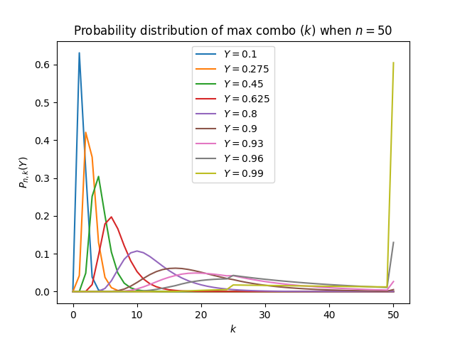
Here are some plots of the probability distribution of max combo <span class="katex"><span class="katex-mathml"><math xmlns="http://www.w3.org/1998/Math/MathML"><semantics><mrow><mi>k</mi></mrow><annotation encoding="application/x-tex">k</annotation></semantics></math></span></span> when <span class="katex"><span class="katex-mathml"><math xmlns="http://www.w3.org/1998/Math/MathML"><semantics><mrow><mi>n</mi><mo>=</mo><mn>50</mn></mrow><annotation encoding="application/x-tex">n=50</annotation></semantics></math></span></span>:</p>
<figure>
<img src="/assets/images/figures/2022-12-25-combo-probability/finite_distribution_50.png" class="dark-adaptive" alt="Probability distribution of  when  for different "/>

</figure>
<p>The plots are intuitive as they show that one has higher probability to get a higher max combo when they have a higher success rate.
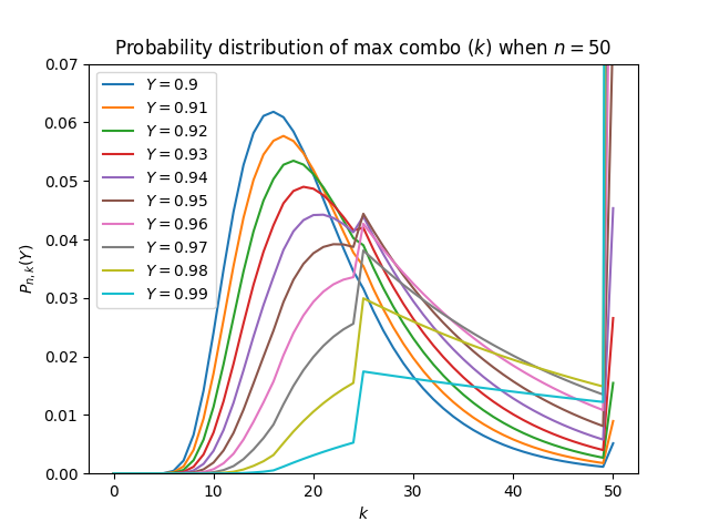
</p>
<p>There is a suspicious jump in <span class="katex"><span class="katex-mathml"><math xmlns="http://www.w3.org/1998/Math/MathML"><semantics><mrow><msub><mi>P</mi><mrow><mi>n</mi><mo separator="true">,</mo><mi>k</mi></mrow></msub><mo stretchy="false">(</mo><mi>Y</mi><mo stretchy="false">)</mo></mrow><annotation encoding="application/x-tex">P_{n,k}(Y)</annotation></semantics></math></span></span> near <span class="katex"><span class="katex-mathml"><math xmlns="http://www.w3.org/1998/Math/MathML"><semantics><mrow><mi>k</mi><mo>=</mo><mi>n</mi><mi mathvariant="normal">/</mi><mn>2</mn></mrow><annotation encoding="application/x-tex">k=n/2</annotation></semantics></math></span></span> when <span class="katex"><span class="katex-mathml"><math xmlns="http://www.w3.org/1998/Math/MathML"><semantics><mrow><mi>Y</mi></mrow><annotation encoding="application/x-tex">Y</annotation></semantics></math></span></span> is close to <span class="katex"><span class="katex-mathml"><math xmlns="http://www.w3.org/1998/Math/MathML"><semantics><mrow><mn>1</mn></mrow><annotation encoding="application/x-tex">1</annotation></semantics></math></span></span>. We can look at it closer:</p>
<figure>
<img src="/assets/images/figures/2022-12-25-combo-probability/finite_distribution_50_2.png" class="dark-adaptive" alt="Probability distribution of  when  for different "/>

</figure>
<p>In the zoomed-in plot, we can also see a jump in first derivative (w.r.t. <span class="katex"><span class="katex-mathml"><math xmlns="http://www.w3.org/1998/Math/MathML"><semantics><mrow><mi>k</mi></mrow><annotation encoding="application/x-tex">k</annotation></semantics></math></span></span>) of <span class="katex"><span class="katex-mathml"><math xmlns="http://www.w3.org/1998/Math/MathML"><semantics><mrow><msub><mi>P</mi><mrow><mi>n</mi><mo separator="true">,</mo><mi>k</mi></mrow></msub><mo stretchy="false">(</mo><mi>Y</mi><mo stretchy="false">)</mo></mrow><annotation encoding="application/x-tex">P_{n,k}(Y)</annotation></semantics></math></span></span> near <span class="katex"><span class="katex-mathml"><math xmlns="http://www.w3.org/1998/Math/MathML"><semantics><mrow><mi>k</mi><mo>=</mo><mi>n</mi><mi mathvariant="normal">/</mi><mn>3</mn></mrow><annotation encoding="application/x-tex">k=n/3</annotation></semantics></math></span></span>. Actually, the jumps can be modeled in later sections when we talk about the case when <span class="katex"><span class="katex-mathml"><math xmlns="http://www.w3.org/1998/Math/MathML"><semantics><mrow><mi>n</mi><mo>→</mo><mi mathvariant="normal">∞</mi></mrow><annotation encoding="application/x-tex">n\to\infty</annotation></semantics></math></span></span>.</p>
<h2 data-label="0.4" id="the-case-when-ntoinfty">The case when <span class="katex"><span class="katex-mathml"><math xmlns="http://www.w3.org/1998/Math/MathML"><semantics><mrow><mi>n</mi><mo>→</mo><mi mathvariant="normal">∞</mi></mrow><annotation encoding="application/x-tex">n\to\infty</annotation></semantics></math></span></span></h2>
<p>A natural approach is to try substituting Equation <a href="#eq:eq-dp2">7</a> into Equation <a href="#eq:eq-f-def">1</a> to get a function w.r.t. the unknown function <span class="katex"><span class="katex-mathml"><math xmlns="http://www.w3.org/1998/Math/MathML"><semantics><mrow><mi>f</mi><mo stretchy="false">(</mo><mi>y</mi><mo separator="true">,</mo><mi>κ</mi><mo stretchy="false">)</mo></mrow><annotation encoding="application/x-tex">f(y,\kappa)</annotation></semantics></math></span></span>. First, we can easily write the case when <span class="katex"><span class="katex-mathml"><math xmlns="http://www.w3.org/1998/Math/MathML"><semantics><mrow><mi>y</mi><mo>=</mo><mn>0</mn></mrow><annotation encoding="application/x-tex">y=0</annotation></semantics></math></span></span> because it means zero success rate, and the only possible max combo is zero: <span id="eq:eq-f-y-0" data-label="(8)"><span class="katex-display-table"> <span class="katex-display-numbered"><span class="katex-display"><span class="katex"><span class="katex-mathml"><math xmlns="http://www.w3.org/1998/Math/MathML" display="block"><semantics><mrow><mi>f</mi><mo stretchy="false">(</mo><mi>y</mi><mo>=</mo><mn>0</mn><mo separator="true">,</mo><mi>κ</mi><mo stretchy="false">)</mo><mo>=</mo><mi>δ</mi><mo stretchy="false">(</mo><mi>κ</mi><mo stretchy="false">)</mo><mi mathvariant="normal">.</mi></mrow><annotation encoding="application/x-tex">f(y=0,\kappa)=\delta(\kappa).</annotation></semantics></math></span></span></span></span> <span class="katex-display-number"><span class="katex-display"><span class="katex"><span class="katex-mathml"><math xmlns="http://www.w3.org/1998/Math/MathML" display="block"><semantics><mrow><mo stretchy="false">(</mo><mn>8</mn><mo stretchy="false">)</mo></mrow><annotation encoding="application/x-tex">(8)</annotation></semantics></math></span></span></span></span> </span></span> Similarly, we can easily write the case when <span class="katex"><span class="katex-mathml"><math xmlns="http://www.w3.org/1998/Math/MathML"><semantics><mrow><mi>y</mi><mo>=</mo><mn>1</mn></mrow><annotation encoding="application/x-tex">y=1</annotation></semantics></math></span></span>: <span id="eq:eq-f-y-1" data-label="(9)"><span class="katex-display-table"> <span class="katex-display-numbered"><span class="katex-display"><span class="katex"><span class="katex-mathml"><math xmlns="http://www.w3.org/1998/Math/MathML" display="block"><semantics><mrow><mi>f</mi><mo stretchy="false">(</mo><mi>y</mi><mo>=</mo><mn>1</mn><mo separator="true">,</mo><mi>κ</mi><mo stretchy="false">)</mo><mo>=</mo><mi>δ</mi><mo stretchy="false">(</mo><mi>κ</mi><mo>−</mo><mn>1</mn><mo stretchy="false">)</mo><mi mathvariant="normal">.</mi></mrow><annotation encoding="application/x-tex">f(y=1,\kappa)=\delta(\kappa-1).</annotation></semantics></math></span></span></span></span> <span class="katex-display-number"><span class="katex-display"><span class="katex"><span class="katex-mathml"><math xmlns="http://www.w3.org/1998/Math/MathML" display="block"><semantics><mrow><mo stretchy="false">(</mo><mn>9</mn><mo stretchy="false">)</mo></mrow><annotation encoding="application/x-tex">(9)</annotation></semantics></math></span></span></span></span> </span></span></p>
<p>From now on, we only consider the case when <span class="katex"><span class="katex-mathml"><math xmlns="http://www.w3.org/1998/Math/MathML"><semantics><mrow><mn>0</mn><mo>&lt;</mo><mi>y</mi><mo>&lt;</mo><mn>1</mn></mrow><annotation encoding="application/x-tex">0&lt;y&lt;1</annotation></semantics></math></span></span>. First, for the case <span class="katex"><span class="katex-mathml"><math xmlns="http://www.w3.org/1998/Math/MathML"><semantics><mrow><mi>κ</mi><mo>=</mo><mn>0</mn></mrow><annotation encoding="application/x-tex">\kappa=0</annotation></semantics></math></span></span>, according to Equation <a href="#eq:eq-dp2">7</a>, <span class="katex-display"><span class="katex"><span class="katex-mathml"><math xmlns="http://www.w3.org/1998/Math/MathML" display="block"><semantics><mtable rowspacing="0.25em" columnalign="right left" columnspacing="0em"><mtr><mtd><mstyle scriptlevel="0" displaystyle="true"><mrow><mi>f</mi><mo stretchy="false">(</mo><mi>y</mi><mo separator="true">,</mo><mi>κ</mi><mo>=</mo><mn>0</mn><mo stretchy="false">)</mo></mrow></mstyle></mtd><mtd><mstyle scriptlevel="0" displaystyle="true"><mrow><mrow/><mo>=</mo><munder><mrow><mi>lim</mi><mo>⁡</mo></mrow><mrow><mi>n</mi><mo>→</mo><mi mathvariant="normal">∞</mi></mrow></munder><mrow><mo fence="true">(</mo><mi>n</mi><mo>+</mo><mn>1</mn><mo fence="true">)</mo></mrow><msup><mrow><mo fence="true">(</mo><mn>1</mn><mo>−</mo><msup><mi>y</mi><mfrac><mn>1</mn><mi>n</mi></mfrac></msup><mo fence="true">)</mo></mrow><mi>n</mi></msup></mrow></mstyle></mtd></mtr><mtr><mtd><mstyle scriptlevel="0" displaystyle="true"><mrow/></mstyle></mtd><mtd><mstyle scriptlevel="0" displaystyle="true"><mrow><mrow/><mo>=</mo><mrow><mo fence="true">{</mo><mtable rowspacing="0.36em" columnalign="left left" columnspacing="1em"><mtr><mtd><mstyle scriptlevel="0" displaystyle="false"><mrow><mn>0</mn><mo separator="true">,</mo></mrow></mstyle></mtd><mtd><mstyle scriptlevel="0" displaystyle="false"><mrow><mn>0</mn><mo>&lt;</mo><mi>y</mi><mo>≤</mo><mn>1</mn><mo separator="true">,</mo></mrow></mstyle></mtd></mtr><mtr><mtd><mstyle scriptlevel="0" displaystyle="false"><mrow><mi mathvariant="normal">∞</mi><mo separator="true">,</mo></mrow></mstyle></mtd><mtd><mstyle scriptlevel="0" displaystyle="false"><mrow><mi>y</mi><mo>=</mo><mn>0.</mn></mrow></mstyle></mtd></mtr></mtable></mrow></mrow></mstyle></mtd></mtr></mtable><annotation encoding="application/x-tex">\begin{align*}
f(y,\kappa=0)&amp;=\lim_{n\to\infty}\left(n+1\right)\left(1-y^{\frac1n}\right)^n\\
&amp;=\begin{cases}0,&amp;0&lt;y\le1,\\\infty,&amp;y=0.\end{cases}
\end{align*}</annotation></semantics></math></span></span></span> The <span class="katex"><span class="katex-mathml"><math xmlns="http://www.w3.org/1998/Math/MathML"><semantics><mrow><mi mathvariant="normal">∞</mi></mrow><annotation encoding="application/x-tex">\infty</annotation></semantics></math></span></span> means that there is a Dirac <span class="katex"><span class="katex-mathml"><math xmlns="http://www.w3.org/1998/Math/MathML"><semantics><mrow><mi>δ</mi></mrow><annotation encoding="application/x-tex">\delta</annotation></semantics></math></span></span> function (shown in Equation <a href="#eq:eq-f-y-0">8</a>).</p>
<p>Then, for the case <span class="katex"><span class="katex-mathml"><math xmlns="http://www.w3.org/1998/Math/MathML"><semantics><mrow><mi>κ</mi><mo>=</mo><mn>1</mn></mrow><annotation encoding="application/x-tex">\kappa=1</annotation></semantics></math></span></span>, according to Equation <a href="#eq:eq-dp2">7</a>, <span class="katex-display"><span class="katex"><span class="katex-mathml"><math xmlns="http://www.w3.org/1998/Math/MathML" display="block"><semantics><mrow><mi>f</mi><mo stretchy="false">(</mo><mi>y</mi><mo separator="true">,</mo><mi>κ</mi><mo>=</mo><mn>1</mn><mo stretchy="false">)</mo><mo>=</mo><munder><mrow><mi>lim</mi><mo>⁡</mo></mrow><mrow><mi>n</mi><mo>→</mo><mi mathvariant="normal">∞</mi></mrow></munder><mrow><mo fence="true">(</mo><mi>n</mi><mo>+</mo><mn>1</mn><mo fence="true">)</mo></mrow><mi>y</mi><mo>=</mo><mi mathvariant="normal">∞</mi><mi mathvariant="normal">.</mi></mrow><annotation encoding="application/x-tex">f(y,\kappa=1)=\lim_{n\to\infty}\left(n+1\right)y=\infty.</annotation></semantics></math></span></span></span> The <span class="katex"><span class="katex-mathml"><math xmlns="http://www.w3.org/1998/Math/MathML"><semantics><mrow><mi mathvariant="normal">∞</mi></mrow><annotation encoding="application/x-tex">\infty</annotation></semantics></math></span></span> means that there is a Dirac <span class="katex"><span class="katex-mathml"><math xmlns="http://www.w3.org/1998/Math/MathML"><semantics><mrow><mi>δ</mi></mrow><annotation encoding="application/x-tex">\delta</annotation></semantics></math></span></span> function. Actually, it is easy to see that there must be a <span class="katex"><span class="katex-mathml"><math xmlns="http://www.w3.org/1998/Math/MathML"><semantics><mrow><mi>y</mi><mi>δ</mi><mo stretchy="false">(</mo><mi>κ</mi><mo>−</mo><mn>1</mn><mo stretchy="false">)</mo></mrow><annotation encoding="application/x-tex">y\delta(\kappa-1)</annotation></semantics></math></span></span> term in the expression of <span class="katex"><span class="katex-mathml"><math xmlns="http://www.w3.org/1998/Math/MathML"><semantics><mrow><mi>f</mi><mo stretchy="false">(</mo><mi>y</mi><mo separator="true">,</mo><mi>κ</mi><mo stretchy="false">)</mo></mrow><annotation encoding="application/x-tex">f(y,\kappa)</annotation></semantics></math></span></span> because the probability of getting a max combo (<span class="katex"><span class="katex-mathml"><math xmlns="http://www.w3.org/1998/Math/MathML"><semantics><mrow><mi>κ</mi><mo>=</mo><mn>1</mn></mrow><annotation encoding="application/x-tex">\kappa=1</annotation></semantics></math></span></span>) is <span class="katex"><span class="katex-mathml"><math xmlns="http://www.w3.org/1998/Math/MathML"><semantics><mrow><mi>y</mi></mrow><annotation encoding="application/x-tex">y</annotation></semantics></math></span></span>.</p>
<p>Define <span id="eq:eq-h-def" data-label="(10)"><span class="katex-display-table"> <span class="katex-display-numbered"><span class="katex-display"><span class="katex"><span class="katex-mathml"><math xmlns="http://www.w3.org/1998/Math/MathML" display="block"><semantics><mrow><mi>h</mi><mo stretchy="false">(</mo><mi>y</mi><mo separator="true">,</mo><mi>κ</mi><mo stretchy="false">)</mo><mo><mi mathvariant="normal">≔</mi></mo><mi>f</mi><mo stretchy="false">(</mo><mi>y</mi><mo separator="true">,</mo><mi>κ</mi><mo stretchy="false">)</mo><mo>−</mo><mi>y</mi><mi>δ</mi><mo stretchy="false">(</mo><mi>κ</mi><mo>−</mo><mn>1</mn><mo stretchy="false">)</mo><mo separator="true">,</mo></mrow><annotation encoding="application/x-tex">h(y,\kappa)\coloneqq f(y,\kappa)-y\delta(\kappa-1),</annotation></semantics></math></span></span></span></span> <span class="katex-display-number"><span class="katex-display"><span class="katex"><span class="katex-mathml"><math xmlns="http://www.w3.org/1998/Math/MathML" display="block"><semantics><mrow><mo stretchy="false">(</mo><mn>10</mn><mo stretchy="false">)</mo></mrow><annotation encoding="application/x-tex">(10)</annotation></semantics></math></span></span></span></span> </span></span> and then we can get rid of the infinity here.</p>
<p>From now on, we only consider the case when <span class="katex"><span class="katex-mathml"><math xmlns="http://www.w3.org/1998/Math/MathML"><semantics><mrow><mn>0</mn><mo>&lt;</mo><mi>y</mi><mo>&lt;</mo><mn>1</mn></mrow><annotation encoding="application/x-tex">0&lt;y&lt;1</annotation></semantics></math></span></span> and <span class="katex"><span class="katex-mathml"><math xmlns="http://www.w3.org/1998/Math/MathML"><semantics><mrow><mn>0</mn><mo>&lt;</mo><mi>κ</mi><mo>&lt;</mo><mn>1</mn></mrow><annotation encoding="application/x-tex">0&lt;\kappa&lt;1</annotation></semantics></math></span></span>. According to Equation <a href="#eq:eq-dp2">7</a>,
<span class="katex-display"><span class="katex"><span class="katex-mathml"><math xmlns="http://www.w3.org/1998/Math/MathML" display="block"><semantics><mtable rowspacing="0.25em" columnalign="right left" columnspacing="0em"><mtr><mtd><mstyle scriptlevel="0" displaystyle="true"><mrow/></mstyle></mtd><mtd><mstyle scriptlevel="0" displaystyle="true"><mrow><mrow/><mphantom><mo>=</mo><mtext> </mtext></mphantom><mi>f</mi><mtext> ⁣</mtext><mrow><mo fence="true">(</mo><mi>y</mi><mo>∈</mo><mrow><mo fence="true">(</mo><mn>0</mn><mo separator="true">,</mo><mn>1</mn><mo fence="true">)</mo></mrow><mo separator="true">,</mo><mi>κ</mi><mo>∈</mo><mrow><mo fence="true">(</mo><mn>0</mn><mo separator="true">,</mo><mn>1</mn><mo fence="true">)</mo></mrow><mo fence="true">)</mo></mrow></mrow></mstyle></mtd></mtr><mtr><mtd><mstyle scriptlevel="0" displaystyle="true"><mrow/></mstyle></mtd><mtd><mstyle scriptlevel="0" displaystyle="true"><mrow><mrow/><mo>=</mo><munder><mrow><mi>lim</mi><mo>⁡</mo></mrow><mrow><mi>n</mi><mo>→</mo><mi mathvariant="normal">∞</mi></mrow></munder><mrow><mo fence="true">(</mo><mi>n</mi><mo>+</mo><mn>1</mn><mo fence="true">)</mo></mrow><mrow><mo fence="true">(</mo><mn>1</mn><mo>−</mo><msup><mi>y</mi><mfrac><mn>1</mn><mi>n</mi></mfrac></msup><mo fence="true">)</mo></mrow><mrow><mo fence="true">(</mo><msup><mi>y</mi><mi>κ</mi></msup><munderover><mo>∑</mo><mrow><msup><mi>k</mi><mo mathvariant="normal" lspace="0em" rspace="0em">′</mo></msup><mo>=</mo><mn>0</mn></mrow><mrow><mi>min</mi><mo>⁡</mo><mo stretchy="false">(</mo><mi>κ</mi><mi>n</mi><mo separator="true">,</mo><mi>n</mi><mo>−</mo><mi>κ</mi><mi>n</mi><mo>−</mo><mn>1</mn><mo stretchy="false">)</mo></mrow></munderover><msub><mi>P</mi><mrow><mi>n</mi><mo>−</mo><mi>κ</mi><mi>n</mi><mo>−</mo><mn>1</mn><mo separator="true">,</mo><msup><mi>k</mi><mo mathvariant="normal" lspace="0em" rspace="0em">′</mo></msup></mrow></msub><mtext> ⁣</mtext><mrow><mo fence="true">(</mo><msup><mi>y</mi><mfrac><mn>1</mn><mi>n</mi></mfrac></msup><mo fence="true">)</mo></mrow></mrow></mrow></mstyle></mtd></mtr><mtr><mtd><mstyle scriptlevel="0" displaystyle="true"><mrow/></mstyle></mtd><mtd><mstyle scriptlevel="0" displaystyle="true"><mrow><mrow/><mphantom><mo>=</mo><munder><mrow><mi>lim</mi><mo>⁡</mo></mrow><mrow><mi>n</mi><mo>→</mo><mi mathvariant="normal">∞</mi></mrow></munder><mrow><mo fence="true">(</mo><mi>n</mi><mo>+</mo><mn>1</mn><mo fence="true">)</mo></mrow><mrow><mo fence="true">(</mo><mn>1</mn><mo>−</mo><msup><mi>y</mi><mfrac><mn>1</mn><mi>n</mi></mfrac></msup><mo fence="true">)</mo></mrow></mphantom><mrow><mo>+</mo><munderover><mo>∑</mo><mrow><mi>r</mi><mo>=</mo><mn>0</mn></mrow><mrow><mi>min</mi><mo>⁡</mo><mo stretchy="false">(</mo><mi>κ</mi><mi>n</mi><mo>−</mo><mn>1</mn><mo separator="true">,</mo><mi>n</mi><mo>−</mo><mi>κ</mi><mi>n</mi><mo>−</mo><mn>1</mn><mo stretchy="false">)</mo></mrow></munderover><msup><mi>y</mi><mfrac><mi>r</mi><mi>n</mi></mfrac></msup><msub><mi>P</mi><mrow><mi>n</mi><mo>−</mo><mi>r</mi><mo>−</mo><mn>1</mn><mo separator="true">,</mo><mi>κ</mi><mi>n</mi></mrow></msub><mtext> ⁣</mtext><mrow><mo fence="true">(</mo><msup><mi>y</mi><mfrac><mn>1</mn><mi>n</mi></mfrac></msup><mo fence="true">)</mo></mrow><mo fence="true">)</mo></mrow></mrow></mstyle></mtd></mtr><mtr><mtd><mstyle scriptlevel="0" displaystyle="true"><mrow/></mstyle></mtd><mtd><mstyle scriptlevel="0" displaystyle="true"><mrow><mrow/><mo>=</mo><munder><mrow><mi>lim</mi><mo>⁡</mo></mrow><mrow><mi>n</mi><mo>→</mo><mi mathvariant="normal">∞</mi></mrow></munder><mi>n</mi><mrow><mo fence="true">(</mo><mn>1</mn><mo>−</mo><msup><mi>y</mi><mfrac><mn>1</mn><mi>n</mi></mfrac></msup><mo fence="true">)</mo></mrow><mo>⋅</mo><munder><mrow><mi>lim</mi><mo>⁡</mo></mrow><mrow><mi>n</mi><mo>→</mo><mi mathvariant="normal">∞</mi></mrow></munder><mrow><mo fence="true">(</mo><msup><mi>y</mi><mi>κ</mi></msup><munderover><mo>∑</mo><mrow><mi>t</mi><mo>=</mo><mn>0</mn><mo separator="true">,</mo><mi mathvariant="normal">Δ</mi><mi>t</mi><mo>=</mo><mfrac><mn>1</mn><mi>n</mi></mfrac></mrow><mrow><mi>min</mi><mo>⁡</mo><mo stretchy="false">(</mo><mi>κ</mi><mo separator="true">,</mo><mn>1</mn><mo>−</mo><mi>κ</mi><mo stretchy="false">)</mo></mrow></munderover><msub><mi>P</mi><mrow><mo stretchy="false">(</mo><mn>1</mn><mo>−</mo><mi>κ</mi><mo stretchy="false">)</mo><mi>n</mi><mo separator="true">,</mo><mi>t</mi><mi>n</mi></mrow></msub><mtext> ⁣</mtext><mrow><mo fence="true">(</mo><msup><mi>y</mi><mfrac><mn>1</mn><mi>n</mi></mfrac></msup><mo fence="true">)</mo></mrow><mo>+</mo><munderover><mo>∑</mo><mrow><mi>t</mi><mo>=</mo><mn>0</mn><mo separator="true">,</mo><mi mathvariant="normal">Δ</mi><mi>t</mi><mo>=</mo><mfrac><mn>1</mn><mi>n</mi></mfrac></mrow><mrow><mi>min</mi><mo>⁡</mo><mo stretchy="false">(</mo><mi>κ</mi><mo separator="true">,</mo><mn>1</mn><mo>−</mo><mi>κ</mi><mo stretchy="false">)</mo></mrow></munderover><msup><mi>y</mi><mi>t</mi></msup><msub><mi>P</mi><mrow><mo stretchy="false">(</mo><mn>1</mn><mo>−</mo><mi>t</mi><mo stretchy="false">)</mo><mi>n</mi><mo separator="true">,</mo><mi>κ</mi><mi>n</mi></mrow></msub><mtext> ⁣</mtext><mrow><mo fence="true">(</mo><msup><mi>y</mi><mfrac><mn>1</mn><mi>n</mi></mfrac></msup><mo fence="true">)</mo></mrow><mo fence="true">)</mo></mrow></mrow></mstyle></mtd></mtr><mtr><mtd><mstyle scriptlevel="0" displaystyle="true"><mrow/></mstyle></mtd><mtd><mstyle scriptlevel="0" displaystyle="true"><mrow><mrow/><mo>=</mo><mo>−</mo><mi>ln</mi><mo>⁡</mo><mi>y</mi><munder><mrow><mi>lim</mi><mo>⁡</mo></mrow><mrow><mi>n</mi><mo>→</mo><mi mathvariant="normal">∞</mi></mrow></munder><mrow><mo fence="true">(</mo><msup><mi>y</mi><mi>κ</mi></msup><munderover><mo>∑</mo><mrow><mi>t</mi><mo>=</mo><mn>0</mn><mo separator="true">,</mo><mi mathvariant="normal">Δ</mi><mi>t</mi><mo>=</mo><mfrac><mn>1</mn><mi>n</mi></mfrac></mrow><mrow><mi>min</mi><mo>⁡</mo><mo stretchy="false">(</mo><mi>κ</mi><mo separator="true">,</mo><mn>1</mn><mo>−</mo><mi>κ</mi><mo stretchy="false">)</mo></mrow></munderover><mfrac><mn>1</mn><mrow><mrow><mo fence="true">(</mo><mn>1</mn><mo>−</mo><mi>κ</mi><mo fence="true">)</mo></mrow><mi>n</mi></mrow></mfrac><mi>f</mi><mtext> ⁣</mtext><mrow><mo fence="true">(</mo><msup><mi>y</mi><mrow><mn>1</mn><mo>−</mo><mi>κ</mi></mrow></msup><mo separator="true">,</mo><mfrac><mi>t</mi><mrow><mn>1</mn><mo>−</mo><mi>κ</mi></mrow></mfrac><mo fence="true">)</mo></mrow></mrow></mrow></mstyle></mtd></mtr><mtr><mtd><mstyle scriptlevel="0" displaystyle="true"><mrow/></mstyle></mtd><mtd><mstyle scriptlevel="0" displaystyle="true"><mrow><mrow/><mphantom><mo>=</mo><mo>−</mo><mi>ln</mi><mo>⁡</mo><mi>y</mi><munder><mrow><mi>lim</mi><mo>⁡</mo></mrow><mrow><mi>n</mi><mo>→</mo><mi mathvariant="normal">∞</mi></mrow></munder></mphantom><mrow><mo>+</mo><munderover><mo>∑</mo><mrow><mi>t</mi><mo>=</mo><mn>0</mn><mo separator="true">,</mo><mi mathvariant="normal">Δ</mi><mi>t</mi><mo>=</mo><mfrac><mn>1</mn><mi>n</mi></mfrac></mrow><mrow><mi>min</mi><mo>⁡</mo><mo stretchy="false">(</mo><mi>κ</mi><mo separator="true">,</mo><mn>1</mn><mo>−</mo><mi>κ</mi><mo stretchy="false">)</mo></mrow></munderover><msup><mi>y</mi><mi>t</mi></msup><mfrac><mn>1</mn><mrow><mrow><mo fence="true">(</mo><mn>1</mn><mo>−</mo><mi>t</mi><mo fence="true">)</mo></mrow><mi>n</mi></mrow></mfrac><mi>f</mi><mtext> ⁣</mtext><mrow><mo fence="true">(</mo><msup><mi>y</mi><mrow><mn>1</mn><mo>−</mo><mi>t</mi></mrow></msup><mo separator="true">,</mo><mfrac><mi>κ</mi><mrow><mn>1</mn><mo>−</mo><mi>t</mi></mrow></mfrac><mo fence="true">)</mo></mrow><mo fence="true">)</mo></mrow></mrow></mstyle></mtd></mtr><mtr><mtd><mstyle scriptlevel="0" displaystyle="true"><mrow/></mstyle></mtd><mtd><mstyle scriptlevel="0" displaystyle="true"><mrow><mrow/><mo>=</mo><mo>−</mo><mi>ln</mi><mo>⁡</mo><mi>y</mi><munder><mrow><mi>lim</mi><mo>⁡</mo></mrow><mrow><mi>n</mi><mo>→</mo><mi mathvariant="normal">∞</mi></mrow></munder><munderover><mo>∑</mo><mrow><mi>t</mi><mo>=</mo><mn>0</mn><mo separator="true">,</mo><mi mathvariant="normal">Δ</mi><mi>t</mi><mo>=</mo><mfrac><mn>1</mn><mi>n</mi></mfrac></mrow><mrow><mi>min</mi><mo>⁡</mo><mo stretchy="false">(</mo><mi>κ</mi><mo separator="true">,</mo><mn>1</mn><mo>−</mo><mi>κ</mi><mo stretchy="false">)</mo></mrow></munderover><mrow><mo fence="true">(</mo><mfrac><msup><mi>y</mi><mi>κ</mi></msup><mrow><mn>1</mn><mo>−</mo><mi>κ</mi></mrow></mfrac><mi>f</mi><mtext> ⁣</mtext><mrow><mo fence="true">(</mo><msup><mi>y</mi><mrow><mn>1</mn><mo>−</mo><mi>κ</mi></mrow></msup><mo separator="true">,</mo><mfrac><mi>t</mi><mrow><mn>1</mn><mo>−</mo><mi>κ</mi></mrow></mfrac><mo fence="true">)</mo></mrow><mo>+</mo><mfrac><msup><mi>y</mi><mi>t</mi></msup><mrow><mn>1</mn><mo>−</mo><mi>t</mi></mrow></mfrac><mi>f</mi><mtext> ⁣</mtext><mrow><mo fence="true">(</mo><msup><mi>y</mi><mrow><mn>1</mn><mo>−</mo><mi>t</mi></mrow></msup><mo separator="true">,</mo><mfrac><mi>κ</mi><mrow><mn>1</mn><mo>−</mo><mi>t</mi></mrow></mfrac><mo fence="true">)</mo></mrow><mo fence="true">)</mo></mrow><mi mathvariant="normal">Δ</mi><mi>t</mi></mrow></mstyle></mtd></mtr><mtr><mtd><mstyle scriptlevel="0" displaystyle="true"><mrow/></mstyle></mtd><mtd><mstyle scriptlevel="0" displaystyle="true"><mrow><mrow/><mo>=</mo><mo>−</mo><mi>ln</mi><mo>⁡</mo><mi>y</mi><msubsup><mo>∫</mo><mrow><mi>t</mi><mo>=</mo><mn>0</mn></mrow><mrow><mi>min</mi><mo>⁡</mo><mo stretchy="false">(</mo><mi>κ</mi><mo separator="true">,</mo><mn>1</mn><mo>−</mo><mi>κ</mi><mo stretchy="false">)</mo></mrow></msubsup><mrow><mo fence="true">(</mo><mfrac><msup><mi>y</mi><mi>κ</mi></msup><mrow><mn>1</mn><mo>−</mo><mi>κ</mi></mrow></mfrac><mi>f</mi><mtext> ⁣</mtext><mrow><mo fence="true">(</mo><msup><mi>y</mi><mrow><mn>1</mn><mo>−</mo><mi>κ</mi></mrow></msup><mo separator="true">,</mo><mfrac><mi>t</mi><mrow><mn>1</mn><mo>−</mo><mi>κ</mi></mrow></mfrac><mo fence="true">)</mo></mrow><mo>+</mo><mfrac><msup><mi>y</mi><mi>t</mi></msup><mrow><mn>1</mn><mo>−</mo><mi>t</mi></mrow></mfrac><mi>f</mi><mtext> ⁣</mtext><mrow><mo fence="true">(</mo><msup><mi>y</mi><mrow><mn>1</mn><mo>−</mo><mi>t</mi></mrow></msup><mo separator="true">,</mo><mfrac><mi>κ</mi><mrow><mn>1</mn><mo>−</mo><mi>t</mi></mrow></mfrac><mo fence="true">)</mo></mrow><mo fence="true">)</mo></mrow><mi mathvariant="normal">d</mi><mi>t</mi><mi mathvariant="normal">.</mi></mrow></mstyle></mtd></mtr></mtable><annotation encoding="application/x-tex">\begin{align*}
&amp;\phantom{=~}f\!\left(y\in\left(0,1\right),\kappa\in\left(0,1\right)\right)\\
&amp;=\lim_{n\to\infty}\left(n+1\right)\left(1-y^{\frac1n}\right)\left(
  y^\kappa\sum_{k'=0}^{\min(\kappa n,n-\kappa n-1)}P_{n-\kappa n-1,k'}\!\left(y^{\frac1n}\right)
\right.\\&amp;\phantom{=\lim_{n\to\infty}\left(n+1\right)\left(1-y^{\frac1n}\right)}\left.
  +\sum_{r=0}^{\min(\kappa n-1,n-\kappa n-1)}y^{\frac rn}P_{n-r-1,\kappa n}\!\left(y^{\frac1n}\right)
\right)\\
&amp;=\lim_{n\to\infty}n\left(1-y^{\frac1n}\right)\cdot\lim_{n\to\infty}\left(
  y^\kappa\sum_{t=0,\Delta t=\frac1n}^{\min(\kappa,1-\kappa)}P_{(1-\kappa)n,tn}\!\left(y^{\frac1n}\right)
  +\sum_{t=0,\Delta t=\frac1n}^{\min(\kappa,1-\kappa)}y^tP_{(1-t)n,\kappa n}\!\left(y^{\frac1n}\right)
\right)\\
&amp;=-\ln y\lim_{n\to\infty}\left(
  y^\kappa\sum_{t=0,\Delta t=\frac1n}^{\min(\kappa,1-\kappa)}
    \frac1{\left(1-\kappa\right)n}f\!\left(y^{1-\kappa},\frac t{1-\kappa}\right)
\right.\\&amp;\phantom{=-\ln y\lim_{n\to\infty}}\left.
  +\sum_{t=0,\Delta t=\frac1n}^{\min(\kappa,1-\kappa)}y^t
    \frac1{\left(1-t\right)n}f\!\left(y^{1-t},\frac{\kappa}{1-t}\right)
\right)\\
&amp;=-\ln y\lim_{n\to\infty}\sum_{t=0,\Delta t=\frac 1n}^{\min(\kappa,1-\kappa)}\left(
  \frac{y^\kappa}{1-\kappa}f\!\left(y^{1-\kappa},\frac t{1-\kappa}\right)
  +\frac{y^t}{1-t}f\!\left(y^{1-t},\frac\kappa{1-t}\right)
\right)\Delta t\\
&amp;=-\ln y\int_{t=0}^{\min(\kappa,1-\kappa)}\left(
  \frac{y^\kappa}{1-\kappa}f\!\left(y^{1-\kappa},\frac t{1-\kappa}\right)
  +\frac{y^t}{1-t}f\!\left(y^{1-t},\frac\kappa{1-t}\right)
\right)\mathrm dt.
\end{align*}</annotation></semantics></math></span></span></span>
Add back the delta function at <span class="katex"><span class="katex-mathml"><math xmlns="http://www.w3.org/1998/Math/MathML"><semantics><mrow><mi>κ</mi><mo>=</mo><mn>1</mn></mrow><annotation encoding="application/x-tex">\kappa=1</annotation></semantics></math></span></span>, and we have the integral equation <span class="katex-display"><span class="katex"><span class="katex-mathml"><math xmlns="http://www.w3.org/1998/Math/MathML" display="block"><semantics><mtable rowspacing="0.25em" columnalign="right left" columnspacing="0em"><mtr><mtd><mstyle scriptlevel="0" displaystyle="true"><mrow><mi>f</mi><mtext> ⁣</mtext><mrow><mo fence="true">(</mo><mi>y</mi><mo>∈</mo><mrow><mo fence="true">(</mo><mn>0</mn><mo separator="true">,</mo><mn>1</mn><mo fence="true">)</mo></mrow><mo separator="true">,</mo><mi>κ</mi><mo fence="true">)</mo></mrow><mo>=</mo><mo>−</mo><mi>ln</mi><mo>⁡</mo><mi>y</mi><msubsup><mo>∫</mo><mrow><mi>t</mi><mo>=</mo><mn>0</mn></mrow><mrow><mi>min</mi><mo>⁡</mo><mo stretchy="false">(</mo><mi>κ</mi><mo separator="true">,</mo><mn>1</mn><mo>−</mo><mi>κ</mi><mo stretchy="false">)</mo></mrow></msubsup></mrow></mstyle></mtd><mtd><mstyle scriptlevel="0" displaystyle="true"><mrow><mrow/><mtext> </mtext><mrow><mo fence="true">(</mo><mfrac><msup><mi>y</mi><mi>κ</mi></msup><mrow><mn>1</mn><mo>−</mo><mi>κ</mi></mrow></mfrac><mi>f</mi><mtext> ⁣</mtext><mrow><mo fence="true">(</mo><msup><mi>y</mi><mrow><mn>1</mn><mo>−</mo><mi>κ</mi></mrow></msup><mo separator="true">,</mo><mfrac><mi>t</mi><mrow><mn>1</mn><mo>−</mo><mi>κ</mi></mrow></mfrac><mo fence="true">)</mo></mrow></mrow></mrow></mstyle></mtd></mtr><mtr><mtd><mstyle scriptlevel="0" displaystyle="true"><mrow/></mstyle></mtd><mtd><mstyle scriptlevel="0" displaystyle="true"><mrow><mrow/><mrow><mo>+</mo><mfrac><msup><mi>y</mi><mi>t</mi></msup><mrow><mn>1</mn><mo>−</mo><mi>t</mi></mrow></mfrac><mi>f</mi><mtext> ⁣</mtext><mrow><mo fence="true">(</mo><msup><mi>y</mi><mrow><mn>1</mn><mo>−</mo><mi>t</mi></mrow></msup><mo separator="true">,</mo><mfrac><mi>κ</mi><mrow><mn>1</mn><mo>−</mo><mi>t</mi></mrow></mfrac><mo fence="true">)</mo></mrow><mo fence="true">)</mo></mrow><mi mathvariant="normal">d</mi><mi>t</mi><mo>+</mo><mi>y</mi><mi>δ</mi><mo stretchy="false">(</mo><mi>κ</mi><mo>−</mo><mn>1</mn><mo stretchy="false">)</mo><mi mathvariant="normal">.</mi></mrow></mstyle></mtd></mtr></mtable><annotation encoding="application/x-tex">\begin{split}
f\!\left(y\in\left(0,1\right),\kappa\right)=-\ln y\int_{t=0}^{\min(\kappa,1-\kappa)}&amp;\,\left(
  \frac{y^\kappa}{1-\kappa}f\!\left(y^{1-\kappa},\frac t{1-\kappa}\right)
\right.\\&amp;\left.
  +\frac{y^t}{1-t}f\!\left(y^{1-t},\frac\kappa{1-t}\right)
\right)\mathrm dt+y\delta(\kappa-1).
\end{split}</annotation></semantics></math></span></span></span></p>
<p>There are two terms in the integral. Substitute <span class="katex"><span class="katex-mathml"><math xmlns="http://www.w3.org/1998/Math/MathML"><semantics><mrow><mi>u</mi><mo><mi mathvariant="normal">≔</mi></mo><mfrac><mi>t</mi><mrow><mn>1</mn><mo>−</mo><mi>κ</mi></mrow></mfrac></mrow><annotation encoding="application/x-tex">u\coloneqq\frac t{1-\kappa}</annotation></semantics></math></span></span> in the first term, and we have <span class="katex-display"><span class="katex"><span class="katex-mathml"><math xmlns="http://www.w3.org/1998/Math/MathML" display="block"><semantics><mtable rowspacing="0.25em" columnalign="right left" columnspacing="0em"><mtr><mtd><mstyle scriptlevel="0" displaystyle="true"><mrow><msubsup><mo>∫</mo><mrow><mi>t</mi><mo>=</mo><mn>0</mn></mrow><mrow><mi>min</mi><mo>⁡</mo><mrow><mo fence="true">(</mo><mi>κ</mi><mo separator="true">,</mo><mn>1</mn><mo>−</mo><mi>κ</mi><mo fence="true">)</mo></mrow></mrow></msubsup><mfrac><msup><mi>y</mi><mi>κ</mi></msup><mrow><mn>1</mn><mo>−</mo><mi>κ</mi></mrow></mfrac><mi>f</mi><mtext> ⁣</mtext><mrow><mo fence="true">(</mo><msup><mi>y</mi><mrow><mn>1</mn><mo>−</mo><mi>κ</mi></mrow></msup><mo separator="true">,</mo><mfrac><mi>t</mi><mrow><mn>1</mn><mo>−</mo><mi>κ</mi></mrow></mfrac><mo fence="true">)</mo></mrow><mi mathvariant="normal">d</mi><mi>t</mi></mrow></mstyle></mtd><mtd><mstyle scriptlevel="0" displaystyle="true"><mrow><mrow/><mo>=</mo><msubsup><mo>∫</mo><mn>0</mn><mrow><mi>min</mi><mo>⁡</mo><mo stretchy="false">(</mo><mfrac><mi>κ</mi><mrow><mn>1</mn><mo>−</mo><mi>κ</mi></mrow></mfrac><mo separator="true">,</mo><mn>1</mn><mo stretchy="false">)</mo></mrow></msubsup><msup><mi>y</mi><mi>κ</mi></msup><mi>f</mi><mtext> ⁣</mtext><mrow><mo fence="true">(</mo><msup><mi>y</mi><mrow><mn>1</mn><mo>−</mo><mi>κ</mi></mrow></msup><mo separator="true">,</mo><mi>u</mi><mo fence="true">)</mo></mrow><mi mathvariant="normal">d</mi><mi>u</mi></mrow></mstyle></mtd></mtr><mtr><mtd><mstyle scriptlevel="0" displaystyle="true"><mrow/></mstyle></mtd><mtd><mstyle scriptlevel="0" displaystyle="true"><mrow><mrow/><mo>=</mo><msubsup><mo>∫</mo><mn>0</mn><mrow><mi>min</mi><mo>⁡</mo><mo stretchy="false">(</mo><mfrac><mi>κ</mi><mrow><mn>1</mn><mo>−</mo><mi>κ</mi></mrow></mfrac><mo separator="true">,</mo><mn>1</mn><mo stretchy="false">)</mo></mrow></msubsup><mrow><mo fence="true">(</mo><msup><mi>y</mi><mi>κ</mi></msup><mi>h</mi><mtext> ⁣</mtext><mrow><mo fence="true">(</mo><msup><mi>y</mi><mrow><mn>1</mn><mo>−</mo><mi>κ</mi></mrow></msup><mo separator="true">,</mo><mi>u</mi><mo fence="true">)</mo></mrow><mo>+</mo><mi>y</mi><mi>δ</mi><mo stretchy="false">(</mo><mi>u</mi><mo>−</mo><mn>1</mn><mo stretchy="false">)</mo><mo fence="true">)</mo></mrow><mi mathvariant="normal">d</mi><mi>u</mi><mi mathvariant="normal">.</mi></mrow></mstyle></mtd></mtr></mtable><annotation encoding="application/x-tex">\begin{align*}
\int_{t=0}^{\min\left(\kappa,1-\kappa\right)}\frac{y^\kappa}{1-\kappa}f\!\left(y^{1-\kappa},\frac t{1-\kappa}\right)\mathrm dt
&amp;=\int_0^{\min(\frac\kappa{1-\kappa},1)}y^\kappa f\!\left(y^{1-\kappa},u\right)\mathrm du\\
&amp;=\int_0^{\min(\frac\kappa{1-\kappa},1)}\left(y^\kappa h\!\left(y^{1-\kappa},u\right)+y\delta(u-1)\right)\mathrm du.
\end{align*}</annotation></semantics></math></span></span></span>
Substitute <span class="katex"><span class="katex-mathml"><math xmlns="http://www.w3.org/1998/Math/MathML"><semantics><mrow><mi>v</mi><mo><mi mathvariant="normal">≔</mi></mo><mfrac><mi>κ</mi><mrow><mn>1</mn><mo>−</mo><mi>t</mi></mrow></mfrac></mrow><annotation encoding="application/x-tex">v\coloneqq\frac\kappa{1-t}</annotation></semantics></math></span></span> in the second term, and we have <span class="katex-display"><span class="katex"><span class="katex-mathml"><math xmlns="http://www.w3.org/1998/Math/MathML" display="block"><semantics><mtable rowspacing="0.25em" columnalign="right left" columnspacing="0em"><mtr><mtd><mstyle scriptlevel="0" displaystyle="true"><mrow><msubsup><mo>∫</mo><mrow><mi>t</mi><mo>=</mo><mn>0</mn></mrow><mrow><mi>min</mi><mo>⁡</mo><mo stretchy="false">(</mo><mi>κ</mi><mo separator="true">,</mo><mn>1</mn><mo>−</mo><mi>κ</mi><mo stretchy="false">)</mo></mrow></msubsup><mfrac><msup><mi>y</mi><mi>t</mi></msup><mrow><mn>1</mn><mo>−</mo><mi>t</mi></mrow></mfrac><mi>f</mi><mtext> ⁣</mtext><mrow><mo fence="true">(</mo><msup><mi>y</mi><mrow><mn>1</mn><mo>−</mo><mi>t</mi></mrow></msup><mo separator="true">,</mo><mfrac><mi>κ</mi><mrow><mn>1</mn><mo>−</mo><mi>t</mi></mrow></mfrac><mo fence="true">)</mo></mrow><mi mathvariant="normal">d</mi><mi>t</mi></mrow></mstyle></mtd><mtd><mstyle scriptlevel="0" displaystyle="true"><mrow><mrow/><mo>=</mo><msubsup><mo>∫</mo><mi>κ</mi><mrow><mi>min</mi><mo>⁡</mo><mrow><mo fence="true">(</mo><mfrac><mi>κ</mi><mrow><mn>1</mn><mo>−</mo><mi>κ</mi></mrow></mfrac><mo separator="true">,</mo><mn>1</mn><mo fence="true">)</mo></mrow></mrow></msubsup><msup><mi>y</mi><mrow><mn>1</mn><mo>−</mo><mfrac><mi>κ</mi><mi>v</mi></mfrac></mrow></msup><mi>f</mi><mtext> ⁣</mtext><mrow><mo fence="true">(</mo><msup><mi>y</mi><mfrac><mi>κ</mi><mi>v</mi></mfrac></msup><mo separator="true">,</mo><mi>v</mi><mo fence="true">)</mo></mrow><mfrac><mrow><mi mathvariant="normal">d</mi><mi>v</mi></mrow><mi>v</mi></mfrac></mrow></mstyle></mtd></mtr><mtr><mtd><mstyle scriptlevel="0" displaystyle="true"><mrow/></mstyle></mtd><mtd><mstyle scriptlevel="0" displaystyle="true"><mrow><mrow/><mo>=</mo><msubsup><mo>∫</mo><mi>κ</mi><mrow><mi>min</mi><mo>⁡</mo><mrow><mo fence="true">(</mo><mfrac><mi>κ</mi><mrow><mn>1</mn><mo>−</mo><mi>κ</mi></mrow></mfrac><mo separator="true">,</mo><mn>1</mn><mo fence="true">)</mo></mrow></mrow></msubsup><mrow><mo fence="true">(</mo><msup><mi>y</mi><mrow><mn>1</mn><mo>−</mo><mfrac><mi>κ</mi><mi>v</mi></mfrac></mrow></msup><mi>h</mi><mtext> ⁣</mtext><mrow><mo fence="true">(</mo><msup><mi>y</mi><mfrac><mi>κ</mi><mi>v</mi></mfrac></msup><mo separator="true">,</mo><mi>v</mi><mo fence="true">)</mo></mrow><mo>+</mo><mi>y</mi><mi>δ</mi><mo stretchy="false">(</mo><mi>v</mi><mo>−</mo><mn>1</mn><mo stretchy="false">)</mo><mo fence="true">)</mo></mrow><mfrac><mrow><mi mathvariant="normal">d</mi><mi>v</mi></mrow><mi>v</mi></mfrac><mi mathvariant="normal">.</mi></mrow></mstyle></mtd></mtr></mtable><annotation encoding="application/x-tex">\begin{align*}
\int_{t=0}^{\min(\kappa,1-\kappa)}\frac{y^t}{1-t}f\!\left(y^{1-t},\frac\kappa{1-t}\right)\mathrm dt
&amp;=\int_\kappa^{\min\left(\frac\kappa{1-\kappa},1\right)}y^{1-\frac\kappa v}f\!\left(y^{\frac\kappa v},v\right)\frac{\mathrm dv}v\\
&amp;=\int_\kappa^{\min\left(\frac\kappa{1-\kappa},1\right)}\left(y^{1-\frac\kappa v}h\!\left(y^{\frac\kappa v},v\right)+y\delta(v-1)\right)\frac{\mathrm dv}v.
\end{align*}</annotation></semantics></math></span></span></span></p>
<p>Further, let (we only consider <span class="katex"><span class="katex-mathml"><math xmlns="http://www.w3.org/1998/Math/MathML"><semantics><mrow><mi>y</mi><mo>∈</mo><mrow><mo fence="true">(</mo><mn>0</mn><mo separator="true">,</mo><mn>1</mn><mo fence="true">)</mo></mrow></mrow><annotation encoding="application/x-tex">y\in\left(0,1\right)</annotation></semantics></math></span></span> from now on) <span id="eq:eq-g-def" data-label="(11)"><span class="katex-display-table"> <span class="katex-display-numbered"><span class="katex-display"><span class="katex"><span class="katex-mathml"><math xmlns="http://www.w3.org/1998/Math/MathML" display="block"><semantics><mrow><mi>g</mi><mo stretchy="false">(</mo><mi>y</mi><mo separator="true">,</mo><mi>κ</mi><mo stretchy="false">)</mo><mo><mi mathvariant="normal">≔</mi></mo><mfrac><mrow><mi>h</mi><mo stretchy="false">(</mo><mi>y</mi><mo separator="true">,</mo><mi>κ</mi><mo stretchy="false">)</mo></mrow><mi>y</mi></mfrac><mo separator="true">,</mo></mrow><annotation encoding="application/x-tex">g(y,\kappa)\coloneqq\frac{h(y,\kappa)}{y},</annotation></semantics></math></span></span></span></span> <span class="katex-display-number"><span class="katex-display"><span class="katex"><span class="katex-mathml"><math xmlns="http://www.w3.org/1998/Math/MathML" display="block"><semantics><mrow><mo stretchy="false">(</mo><mn>11</mn><mo stretchy="false">)</mo></mrow><annotation encoding="application/x-tex">(11)</annotation></semantics></math></span></span></span></span> </span></span> then the integral equation becomes <span id="eq:eq-main" data-label="(12)"><span class="katex-display-table"> <span class="katex-display-numbered"><span class="katex-display"><span class="katex"><span class="katex-mathml"><math xmlns="http://www.w3.org/1998/Math/MathML" display="block"><semantics><mtable rowspacing="0.25em" columnalign="right left" columnspacing="0em"><mtr><mtd><mstyle scriptlevel="0" displaystyle="true"><mrow><mi>g</mi><mo stretchy="false">(</mo><mi>y</mi><mo separator="true">,</mo><mi>κ</mi><mo stretchy="false">)</mo><mo>=</mo><mo>−</mo><mi>ln</mi><mo>⁡</mo><mi>y</mi></mrow></mstyle></mtd><mtd><mstyle scriptlevel="0" displaystyle="true"><mrow><mrow/><mtext> </mtext><mrow><mo fence="true">(</mo><msubsup><mo>∫</mo><mn>0</mn><mrow><mi>min</mi><mo>⁡</mo><mrow><mo fence="true">(</mo><mfrac><mi>κ</mi><mrow><mn>1</mn><mo>−</mo><mi>κ</mi></mrow></mfrac><mo separator="true">,</mo><mn>1</mn><mo fence="true">)</mo></mrow></mrow></msubsup><mrow><mo fence="true">(</mo><mi>g</mi><mtext> ⁣</mtext><mrow><mo fence="true">(</mo><msup><mi>y</mi><mrow><mn>1</mn><mo>−</mo><mi>κ</mi></mrow></msup><mo separator="true">,</mo><mi>u</mi><mo fence="true">)</mo></mrow><mo>+</mo><mi>δ</mi><mo stretchy="false">(</mo><mi>u</mi><mo>−</mo><mn>1</mn><mo stretchy="false">)</mo><mo fence="true">)</mo></mrow><mi mathvariant="normal">d</mi><mi>u</mi></mrow></mrow></mstyle></mtd></mtr><mtr><mtd><mstyle scriptlevel="0" displaystyle="true"><mrow/></mstyle></mtd><mtd><mstyle scriptlevel="0" displaystyle="true"><mrow><mrow/><mrow><mo>+</mo><msubsup><mo>∫</mo><mi>κ</mi><mrow><mi>min</mi><mo>⁡</mo><mrow><mo fence="true">(</mo><mfrac><mi>κ</mi><mrow><mn>1</mn><mo>−</mo><mi>κ</mi></mrow></mfrac><mo separator="true">,</mo><mn>1</mn><mo fence="true">)</mo></mrow></mrow></msubsup><mrow><mo fence="true">(</mo><mi>g</mi><mtext> ⁣</mtext><mrow><mo fence="true">(</mo><msup><mi>y</mi><mfrac><mi>κ</mi><mi>v</mi></mfrac></msup><mo separator="true">,</mo><mi>v</mi><mo fence="true">)</mo></mrow><mo>+</mo><mi>δ</mi><mo stretchy="false">(</mo><mi>v</mi><mo>−</mo><mn>1</mn><mo stretchy="false">)</mo><mo fence="true">)</mo></mrow><mfrac><mrow><mi mathvariant="normal">d</mi><mi>v</mi></mrow><mi>v</mi></mfrac><mo fence="true">)</mo></mrow><mi mathvariant="normal">.</mi></mrow></mstyle></mtd></mtr></mtable><annotation encoding="application/x-tex">\begin{split}
g(y,\kappa)=-\ln y&amp;\,\left(
  \int_0^{\min\left(\frac\kappa{1-\kappa},1\right)}\left(g\!\left(y^{1-\kappa},u\right)+\delta(u-1)\right)\mathrm du
\right.\\&amp;\left.
  +\int_\kappa^{\min\left(\frac\kappa{1-\kappa},1\right)}\left(g\!\left(y^{\frac\kappa v},v\right)+\delta(v-1)\right)\frac{\mathrm dv}v
\right).
\end{split}</annotation></semantics></math></span></span></span></span>
<span class="katex-display-number"><span class="katex-display"><span class="katex"><span class="katex-mathml"><math xmlns="http://www.w3.org/1998/Math/MathML" display="block"><semantics><mrow><mo stretchy="false">(</mo><mn>12</mn><mo stretchy="false">)</mo></mrow><annotation encoding="application/x-tex">(12)</annotation></semantics></math></span></span></span></span> </span></span></p>
<p>There is another integral equation for <span class="katex"><span class="katex-mathml"><math xmlns="http://www.w3.org/1998/Math/MathML"><semantics><mrow><mi>g</mi></mrow><annotation encoding="application/x-tex">g</annotation></semantics></math></span></span>. Because <span class="katex"><span class="katex-mathml"><math xmlns="http://www.w3.org/1998/Math/MathML"><semantics><mrow><msubsup><mo>∫</mo><mn>0</mn><mn>1</mn></msubsup><mi>f</mi><mtext> ⁣</mtext><mrow><mo fence="true">(</mo><mi>y</mi><mo separator="true">,</mo><mi>κ</mi><mo fence="true">)</mo></mrow><mi mathvariant="normal">d</mi><mi>κ</mi><mo>=</mo><mn>1</mn></mrow><annotation encoding="application/x-tex">\int_0^1f\!\left(y,\kappa\right)\mathrm d\kappa=1</annotation></semantics></math></span></span>, we have <span id="eq:eq-normalization" data-label="(13)"><span class="katex-display-table"> <span class="katex-display-numbered"><span class="katex-display"><span class="katex"><span class="katex-mathml"><math xmlns="http://www.w3.org/1998/Math/MathML" display="block"><semantics><mrow><msubsup><mo>∫</mo><mn>0</mn><mn>1</mn></msubsup><mi>g</mi><mtext> ⁣</mtext><mrow><mo fence="true">(</mo><mi>y</mi><mo separator="true">,</mo><mi>κ</mi><mo fence="true">)</mo></mrow><mi mathvariant="normal">d</mi><mi>κ</mi><mo>=</mo><mfrac><mn>1</mn><mi>y</mi></mfrac><mo>−</mo><mn>1.</mn></mrow><annotation encoding="application/x-tex">\int_0^1g\!\left(y,\kappa\right)\mathrm d\kappa=\frac1y-1.</annotation></semantics></math></span></span></span></span> <span class="katex-display-number"><span class="katex-display"><span class="katex"><span class="katex-mathml"><math xmlns="http://www.w3.org/1998/Math/MathML" display="block"><semantics><mrow><mo stretchy="false">(</mo><mn>13</mn><mo stretchy="false">)</mo></mrow><annotation encoding="application/x-tex">(13)</annotation></semantics></math></span></span></span></span> </span></span></p>
<p>Equation <a href="#eq:eq-main">12</a> and <a href="#eq:eq-normalization">13</a> are the equations that we are going to utilize to get the expression for <span class="katex"><span class="katex-mathml"><math xmlns="http://www.w3.org/1998/Math/MathML"><semantics><mrow><mi>g</mi><mo stretchy="false">(</mo><mi>y</mi><mo separator="true">,</mo><mi>κ</mi><mo stretchy="false">)</mo></mrow><annotation encoding="application/x-tex">g(y,\kappa)</annotation></semantics></math></span></span>.</p>
<h3 data-label="0.4.1" id="the-case-kappainleftfrac121right">The case <span class="katex"><span class="katex-mathml"><math xmlns="http://www.w3.org/1998/Math/MathML"><semantics><mrow><mi>κ</mi><mo>∈</mo><mrow><mo fence="true">(</mo><mfrac><mn>1</mn><mn>2</mn></mfrac><mo separator="true">,</mo><mn>1</mn><mo fence="true">)</mo></mrow></mrow><annotation encoding="application/x-tex">\kappa\in\left(\frac12,1\right)</annotation></semantics></math></span></span></h3>
<p>In this case, we have <span class="katex-display"><span class="katex"><span class="katex-mathml"><math xmlns="http://www.w3.org/1998/Math/MathML" display="block"><semantics><mrow><mi>min</mi><mo>⁡</mo><mtext> ⁣</mtext><mrow><mo fence="true">(</mo><mfrac><mi>κ</mi><mrow><mn>1</mn><mo>−</mo><mi>κ</mi></mrow></mfrac><mo separator="true">,</mo><mn>1</mn><mo fence="true">)</mo></mrow><mo>=</mo><mn>1</mn><mo separator="true">,</mo></mrow><annotation encoding="application/x-tex">\min\!\left(\frac\kappa{1-\kappa},1\right)=1,</annotation></semantics></math></span></span></span> so the Dirac delta functions in Equation <a href="#eq:eq-main">12</a> should be considered. In this case, it simplifies to <span id="eq:eq-main-1-2-kappa-1" data-label="(14)"><span class="katex-display-table"> <span class="katex-display-numbered"><span class="katex-display"><span class="katex"><span class="katex-mathml"><math xmlns="http://www.w3.org/1998/Math/MathML" display="block"><semantics><mrow><msub><mi>g</mi><mn>1</mn></msub><mo stretchy="false">(</mo><mi>y</mi><mo separator="true">,</mo><mi>κ</mi><mo stretchy="false">)</mo><mo><mi mathvariant="normal">≔</mi></mo><mi>g</mi><mtext> ⁣</mtext><mrow><mo fence="true">(</mo><mi>y</mi><mo separator="true">,</mo><mi>κ</mi><mo>∈</mo><mrow><mo fence="true">(</mo><mfrac><mn>1</mn><mn>2</mn></mfrac><mo separator="true">,</mo><mn>1</mn><mo fence="true">)</mo></mrow><mo fence="true">)</mo></mrow><mo>=</mo><mo>−</mo><mi>ln</mi><mo>⁡</mo><mi>y</mi><mrow><mo fence="true">(</mo><msup><mi>y</mi><mrow><mi>κ</mi><mo>−</mo><mn>1</mn></mrow></msup><mo>+</mo><msubsup><mo>∫</mo><mi>κ</mi><mn>1</mn></msubsup><mi>g</mi><mtext> ⁣</mtext><mrow><mo fence="true">(</mo><msup><mi>y</mi><mfrac><mi>κ</mi><mi>v</mi></mfrac></msup><mo separator="true">,</mo><mi>v</mi><mo fence="true">)</mo></mrow><mfrac><mrow><mi mathvariant="normal">d</mi><mi>v</mi></mrow><mi>v</mi></mfrac><mo>+</mo><mn>1</mn><mo fence="true">)</mo></mrow><mo separator="true">,</mo></mrow><annotation encoding="application/x-tex">g_1(y,\kappa)\coloneqq g\!\left(y,\kappa\in\left(\frac12,1\right)\right)=
-\ln y\left(y^{\kappa-1}+\int_\kappa^1g\!\left(y^{\frac\kappa v},v\right)\frac{\mathrm dv}v+1\right),</annotation></semantics></math></span></span></span></span> <span class="katex-display-number"><span class="katex-display"><span class="katex"><span class="katex-mathml"><math xmlns="http://www.w3.org/1998/Math/MathML" display="block"><semantics><mrow><mo stretchy="false">(</mo><mn>14</mn><mo stretchy="false">)</mo></mrow><annotation encoding="application/x-tex">(14)</annotation></semantics></math></span></span></span></span> </span></span> where Equation <a href="#eq:eq-normalization">13</a> is utilized when finding the first term.</p>
<p>We can try to solve Equation <a href="#eq:eq-main-1-2-kappa-1">14</a> by using <a href="https://en.wikipedia.org/wiki/Adomian_decomposition_method" target="_blank" rel="external">Adomian decomposition method (ADM)</a>. Suppose <span class="katex"><span class="katex-mathml"><math xmlns="http://www.w3.org/1998/Math/MathML"><semantics><mrow><msub><mi>g</mi><mn>1</mn></msub></mrow><annotation encoding="application/x-tex">g_1</annotation></semantics></math></span></span> can be written in a series <span class="katex-display"><span class="katex"><span class="katex-mathml"><math xmlns="http://www.w3.org/1998/Math/MathML" display="block"><semantics><mrow><msub><mi>g</mi><mn>1</mn></msub><mo>=</mo><msubsup><mi>g</mi><mn>1</mn><mrow><mo stretchy="false">(</mo><mn>0</mn><mo stretchy="false">)</mo></mrow></msubsup><mo>+</mo><msubsup><mi>g</mi><mn>1</mn><mrow><mo stretchy="false">(</mo><mn>1</mn><mo stretchy="false">)</mo></mrow></msubsup><mo>+</mo><mo>⋯</mo><mtext> </mtext><mo separator="true">,</mo></mrow><annotation encoding="application/x-tex">g_1=g_1^{(0)}+g_1^{(1)}+\cdots,</annotation></semantics></math></span></span></span> and substitute it into Equation <a href="#eq:eq-main-1-2-kappa-1">14</a>, and we have <span class="katex-display"><span class="katex"><span class="katex-mathml"><math xmlns="http://www.w3.org/1998/Math/MathML" display="block"><semantics><mrow><msubsup><mi>g</mi><mn>1</mn><mrow><mo stretchy="false">(</mo><mn>0</mn><mo stretchy="false">)</mo></mrow></msubsup><mo stretchy="false">(</mo><mi>y</mi><mo separator="true">,</mo><mi>κ</mi><mo stretchy="false">)</mo><mo>+</mo><mo>⋯</mo><mo>=</mo><mo>−</mo><mi>ln</mi><mo>⁡</mo><mi>y</mi><mrow><mo fence="true">(</mo><msup><mi>y</mi><mrow><mi>κ</mi><mo>−</mo><mn>1</mn></mrow></msup><mo>+</mo><mn>1</mn><mo>+</mo><msubsup><mo>∫</mo><mi>κ</mi><mn>1</mn></msubsup><mrow><mo fence="true">(</mo><msup><mi>g</mi><mrow><mo stretchy="false">(</mo><mn>0</mn><mo stretchy="false">)</mo></mrow></msup><mtext> ⁣</mtext><mrow><mo fence="true">(</mo><msup><mi>y</mi><mfrac><mi>κ</mi><mi>v</mi></mfrac></msup><mo separator="true">,</mo><mi>v</mi><mo fence="true">)</mo></mrow><mo>+</mo><mo>⋯</mo><mtext> </mtext><mo fence="true">)</mo></mrow><mfrac><mrow><mi mathvariant="normal">d</mi><mi>v</mi></mrow><mi>v</mi></mfrac><mo fence="true">)</mo></mrow><mi mathvariant="normal">.</mi></mrow><annotation encoding="application/x-tex">g_1^{(0)}(y,\kappa)+\cdots
=-\ln y\left(y^{\kappa-1}+1+\int_\kappa^1\left(
  g^{(0)}\!\left(y^{\frac\kappa v},v\right)+\cdots
\right)\frac{\mathrm dv}v\right).</annotation></semantics></math></span></span></span> Assume we may interchange integration and summation (which is OK here because we can verify the solution after we find it using ADM). Then,
<span class="katex-display"><span class="katex"><span class="katex-mathml"><math xmlns="http://www.w3.org/1998/Math/MathML" display="block"><semantics><mtable rowspacing="0.25em" columnalign="right left" columnspacing="0em"><mtr><mtd><mstyle scriptlevel="0" displaystyle="true"><mrow/></mstyle></mtd><mtd><mstyle scriptlevel="0" displaystyle="true"><mrow><mrow/><mphantom><mo>=</mo><mtext> </mtext></mphantom><msubsup><mi>g</mi><mn>1</mn><mrow><mo stretchy="false">(</mo><mn>0</mn><mo stretchy="false">)</mo></mrow></msubsup><mo stretchy="false">(</mo><mi>y</mi><mo separator="true">,</mo><mi>κ</mi><mo stretchy="false">)</mo><mo>+</mo><msubsup><mi>g</mi><mn>1</mn><mrow><mo stretchy="false">(</mo><mn>1</mn><mo stretchy="false">)</mo></mrow></msubsup><mo stretchy="false">(</mo><mi>y</mi><mo separator="true">,</mo><mi>κ</mi><mo stretchy="false">)</mo><mo>+</mo><mo>⋯</mo></mrow></mstyle></mtd></mtr><mtr><mtd><mstyle scriptlevel="0" displaystyle="true"><mrow/></mstyle></mtd><mtd><mstyle scriptlevel="0" displaystyle="true"><mrow><mrow/><mo>=</mo><mo>−</mo><mi>ln</mi><mo>⁡</mo><mi>y</mi><mrow><mo fence="true">(</mo><msup><mi>y</mi><mrow><mi>κ</mi><mo>−</mo><mn>1</mn></mrow></msup><mo>+</mo><mn>1</mn><mo fence="true">)</mo></mrow><mo>−</mo><mi>ln</mi><mo>⁡</mo><mi>y</mi><msubsup><mo>∫</mo><mi>κ</mi><mn>1</mn></msubsup><msup><mi>g</mi><mrow><mo stretchy="false">(</mo><mn>0</mn><mo stretchy="false">)</mo></mrow></msup><mtext> ⁣</mtext><mrow><mo fence="true">(</mo><msup><mi>y</mi><mfrac><mi>κ</mi><mi>v</mi></mfrac></msup><mo separator="true">,</mo><mi>v</mi><mo fence="true">)</mo></mrow><mfrac><mrow><mi mathvariant="normal">d</mi><mi>v</mi></mrow><mi>v</mi></mfrac><mo>−</mo><mo>⋯</mo><mtext> </mtext><mi mathvariant="normal">.</mi></mrow></mstyle></mtd></mtr></mtable><annotation encoding="application/x-tex">\begin{align*}
&amp;\phantom{=~}g_1^{(0)}(y,\kappa)+g_1^{(1)}(y,\kappa)+\cdots\\
&amp;=-\ln y\left(y^{\kappa-1}+1\right)
-\ln y\int_\kappa^1g^{(0)}\!\left(y^{\frac\kappa v},v\right)\frac{\mathrm dv}v-\cdots.
\end{align*}</annotation></semantics></math></span></span></span>
If we let <span id="eq:eq-adm-1-2-kappa-1" data-label="(15)"><span class="katex-display-table"> <span class="katex-display-numbered"><span class="katex-display"><span class="katex"><span class="katex-mathml"><math xmlns="http://www.w3.org/1998/Math/MathML" display="block"><semantics><mtable rowspacing="0.25em" columnalign="right left" columnspacing="0em"><mtr><mtd><mstyle scriptlevel="0" displaystyle="true"><mrow><msubsup><mi>g</mi><mn>1</mn><mrow><mo stretchy="false">(</mo><mn>0</mn><mo stretchy="false">)</mo></mrow></msubsup><mo stretchy="false">(</mo><mi>y</mi><mo separator="true">,</mo><mi>κ</mi><mo stretchy="false">)</mo></mrow></mstyle></mtd><mtd><mstyle scriptlevel="0" displaystyle="true"><mrow><mrow/><mo><mi mathvariant="normal">≔</mi></mo><mo>−</mo><mi>ln</mi><mo>⁡</mo><mi>y</mi><mrow><mo fence="true">(</mo><msup><mi>y</mi><mrow><mi>κ</mi><mo>−</mo><mn>1</mn></mrow></msup><mo>+</mo><mn>1</mn><mo fence="true">)</mo></mrow><mo separator="true">,</mo></mrow></mstyle></mtd></mtr><mtr><mtd><mstyle scriptlevel="0" displaystyle="true"><mrow><msubsup><mi>g</mi><mn>1</mn><mrow><mo stretchy="false">(</mo><mi>i</mi><mo>+</mo><mn>1</mn><mo stretchy="false">)</mo></mrow></msubsup><mo stretchy="false">(</mo><mi>y</mi><mo separator="true">,</mo><mi>κ</mi><mo stretchy="false">)</mo></mrow></mstyle></mtd><mtd><mstyle scriptlevel="0" displaystyle="true"><mrow><mrow/><mo><mi mathvariant="normal">≔</mi></mo><mo>−</mo><mi>ln</mi><mo>⁡</mo><mi>y</mi><msubsup><mo>∫</mo><mi>κ</mi><mn>1</mn></msubsup><msup><mi>g</mi><mrow><mo stretchy="false">(</mo><mi>i</mi><mo stretchy="false">)</mo></mrow></msup><mtext> ⁣</mtext><mrow><mo fence="true">(</mo><msup><mi>y</mi><mfrac><mi>κ</mi><mi>v</mi></mfrac></msup><mo separator="true">,</mo><mi>v</mi><mo fence="true">)</mo></mrow><mfrac><mrow><mi mathvariant="normal">d</mi><mi>v</mi></mrow><mi>v</mi></mfrac><mo separator="true">,</mo><mspace width="1em"/><mi>i</mi><mo>∈</mo><mi mathvariant="double-struck">N</mi><mo separator="true">,</mo></mrow></mstyle></mtd></mtr></mtable><annotation encoding="application/x-tex">\begin{split}
g_1^{(0)}(y,\kappa)&amp;\coloneqq-\ln y\left(y^{\kappa-1}+1\right),\\
g_1^{(i+1)}(y,\kappa)&amp;\coloneqq-\ln y\int_\kappa^1g^{(i)}\!\left(y^{\frac\kappa v},v\right)\frac{\mathrm dv}v,\quad i\in\mathbb N,
\end{split}</annotation></semantics></math></span></span></span></span>
<span class="katex-display-number"><span class="katex-display"><span class="katex"><span class="katex-mathml"><math xmlns="http://www.w3.org/1998/Math/MathML" display="block"><semantics><mrow><mo stretchy="false">(</mo><mn>15</mn><mo stretchy="false">)</mo></mrow><annotation encoding="application/x-tex">(15)</annotation></semantics></math></span></span></span></span> </span></span> then we can equate each term in the two series. If the sum <span class="katex"><span class="katex-mathml"><math xmlns="http://www.w3.org/1998/Math/MathML"><semantics><mrow><msub><mi>g</mi><mn>1</mn></msub><mo>=</mo><msubsup><mo>∑</mo><mrow><mi>i</mi><mo>=</mo><mn>0</mn></mrow><mi mathvariant="normal">∞</mi></msubsup><msubsup><mi>g</mi><mn>1</mn><mrow><mo stretchy="false">(</mo><mi>i</mi><mo stretchy="false">)</mo></mrow></msubsup></mrow><annotation encoding="application/x-tex">g_1=\sum_{i=0}^\infty g_1^{(i)}</annotation></semantics></math></span></span> converges, then this is a guess of the solution to Equation <a href="#eq:eq-main-1-2-kappa-1">14</a>, which we can verify whether it is correct or not.</p>
<p>Using Equation <a href="#eq:eq-adm-1-2-kappa-1">15</a>, we can find first few terms in the series by directly integrating. The first few terms are <span class="katex-display"><span class="katex"><span class="katex-mathml"><math xmlns="http://www.w3.org/1998/Math/MathML" display="block"><semantics><mtable rowspacing="0.25em" columnalign="right left" columnspacing="0em"><mtr><mtd><mstyle scriptlevel="0" displaystyle="true"><mrow><msubsup><mi>g</mi><mn>1</mn><mrow><mo stretchy="false">(</mo><mn>0</mn><mo stretchy="false">)</mo></mrow></msubsup><mo stretchy="false">(</mo><mi>y</mi><mo separator="true">,</mo><mi>κ</mi><mo stretchy="false">)</mo></mrow></mstyle></mtd><mtd><mstyle scriptlevel="0" displaystyle="true"><mrow><mrow/><mo>=</mo><mo>−</mo><mi>ln</mi><mo>⁡</mo><mi>y</mi><mrow><mo fence="true">(</mo><msup><mi>y</mi><mrow><mi>κ</mi><mo>−</mo><mn>1</mn></mrow></msup><mo>+</mo><mn>1</mn><mo fence="true">)</mo></mrow><mo separator="true">,</mo></mrow></mstyle></mtd></mtr><mtr><mtd><mstyle scriptlevel="0" displaystyle="true"><mrow><msubsup><mi>g</mi><mn>1</mn><mrow><mo stretchy="false">(</mo><mn>1</mn><mo stretchy="false">)</mo></mrow></msubsup><mo stretchy="false">(</mo><mi>y</mi><mo separator="true">,</mo><mi>κ</mi><mo stretchy="false">)</mo></mrow></mstyle></mtd><mtd><mstyle scriptlevel="0" displaystyle="true"><mrow><mrow/><mo>=</mo><mo>−</mo><mi>ln</mi><mo>⁡</mo><mi>y</mi><mrow><mo fence="true">(</mo><msup><mi>y</mi><mrow><mi>κ</mi><mo>−</mo><mn>1</mn></mrow></msup><mo>−</mo><mn>1</mn><mo>+</mo><mi>ln</mi><mo>⁡</mo><msup><mi>y</mi><mrow><mi>κ</mi><mo>−</mo><mn>1</mn></mrow></msup><mo fence="true">)</mo></mrow><mo separator="true">,</mo></mrow></mstyle></mtd></mtr><mtr><mtd><mstyle scriptlevel="0" displaystyle="true"><mrow><msubsup><mi>g</mi><mn>1</mn><mrow><mo stretchy="false">(</mo><mn>2</mn><mo stretchy="false">)</mo></mrow></msubsup><mo stretchy="false">(</mo><mi>y</mi><mo separator="true">,</mo><mi>κ</mi><mo stretchy="false">)</mo></mrow></mstyle></mtd><mtd><mstyle scriptlevel="0" displaystyle="true"><mrow><mrow/><mo>=</mo><mo>−</mo><mi>ln</mi><mo>⁡</mo><mi>y</mi><mrow><mo fence="true">(</mo><msup><mi>y</mi><mrow><mi>κ</mi><mo>−</mo><mn>1</mn></mrow></msup><mo>−</mo><mn>1</mn><mo>−</mo><mi>ln</mi><mo>⁡</mo><msup><mi>y</mi><mrow><mi>κ</mi><mo>−</mo><mn>1</mn></mrow></msup><mo>+</mo><mfrac><mn>1</mn><mn>2</mn></mfrac><msup><mrow><mo fence="true">(</mo><mi>ln</mi><mo>⁡</mo><msup><mi>y</mi><mrow><mi>κ</mi><mo>−</mo><mn>1</mn></mrow></msup><mo fence="true">)</mo></mrow><mn>2</mn></msup><mo fence="true">)</mo></mrow><mo separator="true">,</mo></mrow></mstyle></mtd></mtr><mtr><mtd><mstyle scriptlevel="0" displaystyle="true"><mrow><msubsup><mi>g</mi><mn>1</mn><mrow><mo stretchy="false">(</mo><mn>3</mn><mo stretchy="false">)</mo></mrow></msubsup><mo stretchy="false">(</mo><mi>y</mi><mo separator="true">,</mo><mi>κ</mi><mo stretchy="false">)</mo></mrow></mstyle></mtd><mtd><mstyle scriptlevel="0" displaystyle="true"><mrow><mrow/><mo>=</mo><mo>−</mo><mi>ln</mi><mo>⁡</mo><mi>y</mi><mrow><mo fence="true">(</mo><msup><mi>y</mi><mrow><mi>κ</mi><mo>−</mo><mn>1</mn></mrow></msup><mo>−</mo><mn>1</mn><mo>−</mo><mi>ln</mi><mo>⁡</mo><msup><mi>y</mi><mrow><mi>κ</mi><mo>−</mo><mn>1</mn></mrow></msup><mo>−</mo><mfrac><mn>1</mn><mn>2</mn></mfrac><msup><mrow><mo fence="true">(</mo><mi>ln</mi><mo>⁡</mo><msup><mi>y</mi><mrow><mi>κ</mi><mo>−</mo><mn>1</mn></mrow></msup><mo fence="true">)</mo></mrow><mn>2</mn></msup><mo>+</mo><mfrac><mn>1</mn><mn>6</mn></mfrac><msup><mrow><mo fence="true">(</mo><mi>ln</mi><mo>⁡</mo><msup><mi>y</mi><mrow><mi>κ</mi><mo>−</mo><mn>1</mn></mrow></msup><mo fence="true">)</mo></mrow><mn>3</mn></msup><mo fence="true">)</mo></mrow><mo separator="true">,</mo></mrow></mstyle></mtd></mtr><mtr><mtd><mstyle scriptlevel="0" displaystyle="true"><mi><mi mathvariant="normal">⋮</mi><mpadded height="0em" voffset="0em"><mspace mathbackground="black" width="0em" height="1.5em"/></mpadded></mi></mstyle></mtd><mtd><mstyle scriptlevel="0" displaystyle="true"><mrow/></mstyle></mtd></mtr></mtable><annotation encoding="application/x-tex">\begin{split}
g_1^{(0)}(y,\kappa)&amp;=-\ln y\left(y^{\kappa-1}+1\right),\\
g_1^{(1)}(y,\kappa)&amp;=-\ln y\left(y^{\kappa-1}-1+\ln y^{\kappa-1}\right),\\
g_1^{(2)}(y,\kappa)&amp;=-\ln y\left(y^{\kappa-1}-1-\ln y^{\kappa-1}+\frac12\left(\ln y^{\kappa-1}\right)^2\right),\\
g_1^{(3)}(y,\kappa)&amp;=-\ln y\left(y^{\kappa-1}-1-\ln y^{\kappa-1}-\frac12\left(\ln y^{\kappa-1}\right)^2+\frac16\left(\ln y^{\kappa-1}\right)^3\right),\\
\vdots&amp;
\end{split}</annotation></semantics></math></span></span></span>
We may then guess that the terms have general formula <span class="katex-display"><span class="katex"><span class="katex-mathml"><math xmlns="http://www.w3.org/1998/Math/MathML" display="block"><semantics><mrow><msubsup><mi>g</mi><mn>1</mn><mrow><mo stretchy="false">(</mo><mi>i</mi><mo stretchy="false">)</mo></mrow></msubsup><mo stretchy="false">(</mo><mi>y</mi><mo separator="true">,</mo><mi>κ</mi><mo stretchy="false">)</mo><mo>=</mo><mo>−</mo><mi>ln</mi><mo>⁡</mo><mi>y</mi><mrow><mo fence="true">(</mo><msup><mi>y</mi><mrow><mi>κ</mi><mo>−</mo><mn>1</mn></mrow></msup><mo>+</mo><mfrac><mn>1</mn><mrow><mi>i</mi><mo stretchy="false">!</mo></mrow></mfrac><msup><mrow><mo fence="true">(</mo><mi>ln</mi><mo>⁡</mo><msup><mi>y</mi><mrow><mi>κ</mi><mo>−</mo><mn>1</mn></mrow></msup><mo fence="true">)</mo></mrow><mi>i</mi></msup><mo>−</mo><munderover><mo>∑</mo><mrow><mi>j</mi><mo>=</mo><mn>0</mn></mrow><mrow><mi>i</mi><mo>−</mo><mn>1</mn></mrow></munderover><mfrac><mn>1</mn><mrow><mi>j</mi><mo stretchy="false">!</mo></mrow></mfrac><msup><mrow><mo fence="true">(</mo><mi>ln</mi><mo>⁡</mo><msup><mi>y</mi><mrow><mi>κ</mi><mo>−</mo><mn>1</mn></mrow></msup><mo fence="true">)</mo></mrow><mi>j</mi></msup><mo fence="true">)</mo></mrow><mi mathvariant="normal">.</mi></mrow><annotation encoding="application/x-tex">g_1^{(i)}(y,\kappa)=-\ln y\left(y^{\kappa-1}+\frac1{i!}\left(\ln y^{\kappa-1}\right)^i
-\sum_{j=0}^{i-1}\frac1{j!}\left(\ln y^{\kappa-1}\right)^j\right).</annotation></semantics></math></span></span></span> Sum up the terms, and we have
<span class="katex-display"><span class="katex"><span class="katex-mathml"><math xmlns="http://www.w3.org/1998/Math/MathML" display="block"><semantics><mtable rowspacing="0.25em" columnalign="right left" columnspacing="0em"><mtr><mtd><mstyle scriptlevel="0" displaystyle="true"><mrow><msub><mi>g</mi><mn>1</mn></msub><mo stretchy="false">(</mo><mi>y</mi><mo separator="true">,</mo><mi>κ</mi><mo stretchy="false">)</mo></mrow></mstyle></mtd><mtd><mstyle scriptlevel="0" displaystyle="true"><mrow><mrow/><mo>=</mo><munderover><mo>∑</mo><mrow><mi>i</mi><mo>=</mo><mn>0</mn></mrow><mi mathvariant="normal">∞</mi></munderover><msubsup><mi>g</mi><mn>1</mn><mrow><mo stretchy="false">(</mo><mi>i</mi><mo stretchy="false">)</mo></mrow></msubsup><mo stretchy="false">(</mo><mi>y</mi><mo separator="true">,</mo><mi>κ</mi><mo stretchy="false">)</mo></mrow></mstyle></mtd></mtr><mtr><mtd><mstyle scriptlevel="0" displaystyle="true"><mrow/></mstyle></mtd><mtd><mstyle scriptlevel="0" displaystyle="true"><mrow><mrow/><mo>=</mo><munder><mrow><mi>lim</mi><mo>⁡</mo></mrow><mrow><mi>q</mi><mo>→</mo><mi mathvariant="normal">∞</mi></mrow></munder><munderover><mo>∑</mo><mrow><mi>i</mi><mo>=</mo><mn>0</mn></mrow><mi>q</mi></munderover><mo>−</mo><mi>ln</mi><mo>⁡</mo><mi>y</mi><mrow><mo fence="true">(</mo><msup><mi>y</mi><mrow><mi>κ</mi><mo>−</mo><mn>1</mn></mrow></msup><mo>+</mo><mfrac><mn>1</mn><mrow><mi>i</mi><mo stretchy="false">!</mo></mrow></mfrac><msup><mrow><mo fence="true">(</mo><mi>ln</mi><mo>⁡</mo><msup><mi>y</mi><mrow><mi>κ</mi><mo>−</mo><mn>1</mn></mrow></msup><mo fence="true">)</mo></mrow><mi>i</mi></msup><mo>−</mo><munderover><mo>∑</mo><mrow><mi>j</mi><mo>=</mo><mn>0</mn></mrow><mrow><mi>i</mi><mo>−</mo><mn>1</mn></mrow></munderover><mfrac><mn>1</mn><mrow><mi>j</mi><mo stretchy="false">!</mo></mrow></mfrac><msup><mrow><mo fence="true">(</mo><mi>ln</mi><mo>⁡</mo><msup><mi>y</mi><mrow><mi>κ</mi><mo>−</mo><mn>1</mn></mrow></msup><mo fence="true">)</mo></mrow><mi>j</mi></msup><mo fence="true">)</mo></mrow></mrow></mstyle></mtd></mtr><mtr><mtd><mstyle scriptlevel="0" displaystyle="true"><mrow/></mstyle></mtd><mtd><mstyle scriptlevel="0" displaystyle="true"><mrow><mrow/><mo>=</mo><mo>−</mo><mi>ln</mi><mo>⁡</mo><mi>y</mi><mrow><mo fence="true">(</mo><mi>exp</mi><mo>⁡</mo><mi>ln</mi><mo>⁡</mo><msup><mi>y</mi><mrow><mi>κ</mi><mo>−</mo><mn>1</mn></mrow></msup><mo>+</mo><munder><mrow><mi>lim</mi><mo>⁡</mo></mrow><mrow><mi>q</mi><mo>→</mo><mi mathvariant="normal">∞</mi></mrow></munder><mrow><mo fence="true">(</mo><mrow><mo fence="true">(</mo><mi>q</mi><mo>+</mo><mn>1</mn><mo fence="true">)</mo></mrow><msup><mi>y</mi><mrow><mi>κ</mi><mo>−</mo><mn>1</mn></mrow></msup><mo>−</mo><munderover><mo>∑</mo><mrow><mi>j</mi><mo>=</mo><mn>0</mn></mrow><mi>q</mi></munderover><munderover><mo>∑</mo><mrow><mi>i</mi><mo>=</mo><mi>j</mi><mo>+</mo><mn>1</mn></mrow><mi>q</mi></munderover><mfrac><mn>1</mn><mrow><mi>j</mi><mo stretchy="false">!</mo></mrow></mfrac><msup><mrow><mo fence="true">(</mo><mi>ln</mi><mo>⁡</mo><msup><mi>y</mi><mrow><mi>κ</mi><mo>−</mo><mn>1</mn></mrow></msup><mo fence="true">)</mo></mrow><mi>j</mi></msup><mo fence="true">)</mo></mrow><mo fence="true">)</mo></mrow></mrow></mstyle></mtd></mtr><mtr><mtd><mstyle scriptlevel="0" displaystyle="true"><mrow/></mstyle></mtd><mtd><mstyle scriptlevel="0" displaystyle="true"><mrow><mrow/><mo>=</mo><mo>−</mo><mi>ln</mi><mo>⁡</mo><mi>y</mi><mrow><mo fence="true">(</mo><msup><mi>y</mi><mrow><mi>κ</mi><mo>−</mo><mn>1</mn></mrow></msup><mo>+</mo><munder><mrow><mi>lim</mi><mo>⁡</mo></mrow><mrow><mi>q</mi><mo>→</mo><mi mathvariant="normal">∞</mi></mrow></munder><mrow><mo fence="true">(</mo><mrow><mo fence="true">(</mo><mi>q</mi><mo>+</mo><mn>1</mn><mo fence="true">)</mo></mrow><msup><mi>y</mi><mrow><mi>κ</mi><mo>−</mo><mn>1</mn></mrow></msup><mo>−</mo><munderover><mo>∑</mo><mrow><mi>j</mi><mo>=</mo><mn>0</mn></mrow><mi>q</mi></munderover><mfrac><mrow><mi>q</mi><mo>−</mo><mi>j</mi></mrow><mrow><mi>j</mi><mo stretchy="false">!</mo></mrow></mfrac><msup><mrow><mo fence="true">(</mo><mi>ln</mi><mo>⁡</mo><msup><mi>y</mi><mrow><mi>κ</mi><mo>−</mo><mn>1</mn></mrow></msup><mo fence="true">)</mo></mrow><mi>j</mi></msup><mo fence="true">)</mo></mrow><mo fence="true">)</mo></mrow></mrow></mstyle></mtd></mtr><mtr><mtd><mstyle scriptlevel="0" displaystyle="true"><mrow/></mstyle></mtd><mtd><mstyle scriptlevel="0" displaystyle="true"><mrow><mrow/><mo>=</mo><mo>−</mo><mi>ln</mi><mo>⁡</mo><mi>y</mi><mrow><mo fence="true">(</mo><msup><mi>y</mi><mrow><mi>κ</mi><mo>−</mo><mn>1</mn></mrow></msup><mo>+</mo><munder><mrow><mi>lim</mi><mo>⁡</mo></mrow><mrow><mi>q</mi><mo>→</mo><mi mathvariant="normal">∞</mi></mrow></munder><mrow><mo fence="true">(</mo><mi>q</mi><msup><mi>y</mi><mrow><mi>κ</mi><mo>−</mo><mn>1</mn></mrow></msup><mo>−</mo><mi>q</mi><munderover><mo>∑</mo><mrow><mi>j</mi><mo>=</mo><mn>0</mn></mrow><mi>q</mi></munderover><mfrac><mn>1</mn><mrow><mi>j</mi><mo stretchy="false">!</mo></mrow></mfrac><msup><mrow><mo fence="true">(</mo><mi>ln</mi><mo>⁡</mo><msup><mi>y</mi><mrow><mi>κ</mi><mo>−</mo><mn>1</mn></mrow></msup><mo fence="true">)</mo></mrow><mi>j</mi></msup><mo fence="true">)</mo></mrow></mrow></mrow></mstyle></mtd></mtr><mtr><mtd><mstyle scriptlevel="0" displaystyle="true"><mrow/></mstyle></mtd><mtd><mstyle scriptlevel="0" displaystyle="true"><mrow><mrow/><mphantom><mo>=</mo><mo>−</mo><mi>ln</mi><mo>⁡</mo><mi>y</mi></mphantom><mrow><mpadded width="0px"><mphantom><munderover><mo>∑</mo><mi>j</mi><mi>q</mi></munderover></mphantom></mpadded><mo>+</mo><msup><mi>y</mi><mrow><mi>κ</mi><mo>−</mo><mn>1</mn></mrow></msup><mo>+</mo><mi>ln</mi><mo>⁡</mo><msup><mi>y</mi><mrow><mi>κ</mi><mo>−</mo><mn>1</mn></mrow></msup><mi>exp</mi><mo>⁡</mo><mi>ln</mi><mo>⁡</mo><msup><mi>y</mi><mrow><mi>κ</mi><mo>−</mo><mn>1</mn></mrow></msup><mo fence="true">)</mo></mrow></mrow></mstyle></mtd></mtr><mtr><mtd><mstyle scriptlevel="0" displaystyle="true"><mrow/></mstyle></mtd><mtd><mstyle scriptlevel="0" displaystyle="true"><mrow><mrow/><mo>=</mo><mo>−</mo><mi>ln</mi><mo>⁡</mo><mi>y</mi><mrow><mo fence="true">(</mo><mn>2</mn><mo>+</mo><mi>ln</mi><mo>⁡</mo><msup><mi>y</mi><mrow><mi>κ</mi><mo>−</mo><mn>1</mn></mrow></msup><mo fence="true">)</mo></mrow><msup><mi>y</mi><mrow><mi>κ</mi><mo>−</mo><mn>1</mn></mrow></msup><mi mathvariant="normal">.</mi></mrow></mstyle></mtd></mtr></mtable><annotation encoding="application/x-tex">\begin{align*}
g_1(y,\kappa)&amp;=\sum_{i=0}^\infty g_1^{(i)}(y,\kappa)\\
&amp;=\lim_{q\to\infty}\sum_{i=0}^q-\ln y\left(
  y^{\kappa-1}+\frac1{i!}\left(\ln y^{\kappa-1}\right)^i
  -\sum_{j=0}^{i-1}\frac1{j!}\left(\ln y^{\kappa-1}\right)^j
\right)\\
&amp;=-\ln y\left(\exp\ln y^{\kappa-1}+\lim_{q\to\infty}\left(
  \left(q+1\right)y^{\kappa-1}
  -\sum_{j=0}^q\sum_{i=j+1}^q\frac1{j!}\left(\ln y^{\kappa-1}\right)^j
\right)\right)\\
&amp;=-\ln y\left(y^{\kappa-1}+\lim_{q\to\infty}\left(
  \left(q+1\right)y^{\kappa-1}
  -\sum_{j=0}^q\frac{q-j}{j!}\left(\ln y^{\kappa-1}\right)^j
\right)\right)\\
&amp;=-\ln y\left(
  y^{\kappa-1}+\lim_{q\to\infty}\left(
    qy^{\kappa-1}-q\sum_{j=0}^q\frac1{j!}\left(\ln y^{\kappa-1}\right)^j
  \right)
\right.\\&amp;\phantom{=-\ln y}\left.\vphantom{\sum_j^q}
  +y^{\kappa-1}
  +\ln y^{\kappa-1}\exp\ln y^{\kappa-1}
\right)\\
&amp;=-\ln y\left(2+\ln y^{\kappa-1}\right)y^{\kappa-1}.
\end{align*}</annotation></semantics></math></span></span></span></p>
<p>Therefore, we have the final guess of solution <span id="eq:eq-g1" data-label="(16)"><span class="katex-display-table"> <span class="katex-display-numbered"><span class="katex-display"><span class="katex"><span class="katex-mathml"><math xmlns="http://www.w3.org/1998/Math/MathML" display="block"><semantics><mrow><msub><mi>g</mi><mn>1</mn></msub><mo stretchy="false">(</mo><mi>y</mi><mo separator="true">,</mo><mi>κ</mi><mo stretchy="false">)</mo><mo>=</mo><mo>−</mo><mi>ln</mi><mo>⁡</mo><mi>y</mi><mrow><mo fence="true">(</mo><mn>2</mn><mo>+</mo><mi>ln</mi><mo>⁡</mo><msup><mi>y</mi><mrow><mi>κ</mi><mo>−</mo><mn>1</mn></mrow></msup><mo fence="true">)</mo></mrow><msup><mi>y</mi><mrow><mi>κ</mi><mo>−</mo><mn>1</mn></mrow></msup><mi mathvariant="normal">.</mi></mrow><annotation encoding="application/x-tex">g_1(y,\kappa)=-\ln y\left(2+\ln y^{\kappa-1}\right)y^{\kappa-1}.</annotation></semantics></math></span></span></span></span> <span class="katex-display-number"><span class="katex-display"><span class="katex"><span class="katex-mathml"><math xmlns="http://www.w3.org/1998/Math/MathML" display="block"><semantics><mrow><mo stretchy="false">(</mo><mn>16</mn><mo stretchy="false">)</mo></mrow><annotation encoding="application/x-tex">(16)</annotation></semantics></math></span></span></span></span> </span></span> We can substitute it into Equation <a href="#eq:eq-main-1-2-kappa-1">14</a> to verify that it is indeed the solution.</p>
<h3 data-label="0.4.2" id="the-case-kappainleftfrac13frac12right">The case <span class="katex"><span class="katex-mathml"><math xmlns="http://www.w3.org/1998/Math/MathML"><semantics><mrow><mi>κ</mi><mo>∈</mo><mrow><mo fence="true">(</mo><mfrac><mn>1</mn><mn>3</mn></mfrac><mo separator="true">,</mo><mfrac><mn>1</mn><mn>2</mn></mfrac><mo fence="true">)</mo></mrow></mrow><annotation encoding="application/x-tex">\kappa\in\left(\frac13,\frac12\right)</annotation></semantics></math></span></span></h3>
<p>In this case, we have <span class="katex-display"><span class="katex"><span class="katex-mathml"><math xmlns="http://www.w3.org/1998/Math/MathML" display="block"><semantics><mrow><mi>min</mi><mo>⁡</mo><mtext> ⁣</mtext><mrow><mo fence="true">(</mo><mfrac><mi>κ</mi><mrow><mn>1</mn><mo>−</mo><mi>κ</mi></mrow></mfrac><mo separator="true">,</mo><mn>1</mn><mo fence="true">)</mo></mrow><mo>=</mo><mfrac><mi>κ</mi><mrow><mn>1</mn><mo>−</mo><mi>κ</mi></mrow></mfrac><mo>∈</mo><mrow><mo fence="true">(</mo><mfrac><mn>1</mn><mn>2</mn></mfrac><mo separator="true">,</mo><mn>1</mn><mo fence="true">)</mo></mrow><mi mathvariant="normal">.</mi></mrow><annotation encoding="application/x-tex">\min\!\left(\frac\kappa{1-\kappa},1\right)=\frac\kappa{1-\kappa}\in\left(\frac12,1\right).</annotation></semantics></math></span></span></span> We can then use the same method as in the previous case to find the solution.</p>
<p>First, by Equation <a href="#eq:eq-main-1-2-kappa-1">14</a>, <span class="katex-display"><span class="katex"><span class="katex-mathml"><math xmlns="http://www.w3.org/1998/Math/MathML" display="block"><semantics><mtable rowspacing="0.25em" columnalign="right left" columnspacing="0em"><mtr><mtd><mstyle scriptlevel="0" displaystyle="true"><mrow><msub><mi>g</mi><mn>2</mn></msub><mo stretchy="false">(</mo><mi>y</mi><mo separator="true">,</mo><mi>κ</mi><mo stretchy="false">)</mo></mrow></mstyle></mtd><mtd><mstyle scriptlevel="0" displaystyle="true"><mrow><mrow/><mo><mi mathvariant="normal">≔</mi></mo><mi>g</mi><mtext> ⁣</mtext><mrow><mo fence="true">(</mo><mi>y</mi><mo separator="true">,</mo><mi>κ</mi><mo>∈</mo><mrow><mo fence="true">(</mo><mfrac><mn>1</mn><mn>3</mn></mfrac><mo separator="true">,</mo><mfrac><mn>1</mn><mn>2</mn></mfrac><mo fence="true">)</mo></mrow><mo fence="true">)</mo></mrow></mrow></mstyle></mtd></mtr><mtr><mtd><mstyle scriptlevel="0" displaystyle="true"><mrow/></mstyle></mtd><mtd><mstyle scriptlevel="0" displaystyle="true"><mrow><mrow/><mo>=</mo><mo>−</mo><mi>ln</mi><mo>⁡</mo><mi>y</mi><mrow><mo fence="true">(</mo><msubsup><mo>∫</mo><mn>0</mn><mfrac><mi>κ</mi><mrow><mn>1</mn><mo>−</mo><mi>κ</mi></mrow></mfrac></msubsup><mi>g</mi><mtext> ⁣</mtext><mrow><mo fence="true">(</mo><msup><mi>y</mi><mrow><mn>1</mn><mo>−</mo><mi>κ</mi></mrow></msup><mo separator="true">,</mo><mi>u</mi><mo fence="true">)</mo></mrow><mi mathvariant="normal">d</mi><mi>u</mi><mo>+</mo><msubsup><mo>∫</mo><mi>κ</mi><mfrac><mi>κ</mi><mrow><mn>1</mn><mo>−</mo><mi>κ</mi></mrow></mfrac></msubsup><mi>g</mi><mtext> ⁣</mtext><mrow><mo fence="true">(</mo><msup><mi>y</mi><mfrac><mi>κ</mi><mi>v</mi></mfrac></msup><mo separator="true">,</mo><mi>v</mi><mo fence="true">)</mo></mrow><mfrac><mrow><mi mathvariant="normal">d</mi><mi>v</mi></mrow><mi>v</mi></mfrac><mo fence="true">)</mo></mrow></mrow></mstyle></mtd></mtr><mtr><mtd><mstyle scriptlevel="0" displaystyle="true"><mrow/></mstyle></mtd><mtd><mstyle scriptlevel="0" displaystyle="true"><mrow><mrow/><mo>=</mo><mo>−</mo><mi>ln</mi><mo>⁡</mo><mi>y</mi><mrow><mo fence="true">(</mo><msubsup><mo>∫</mo><mn>0</mn><mn>1</mn></msubsup><mi>g</mi><mtext> ⁣</mtext><mrow><mo fence="true">(</mo><msup><mi>y</mi><mrow><mn>1</mn><mo>−</mo><mi>κ</mi></mrow></msup><mo separator="true">,</mo><mi>u</mi><mo fence="true">)</mo></mrow><mi mathvariant="normal">d</mi><mi>u</mi><mo>−</mo><msubsup><mo>∫</mo><mfrac><mi>κ</mi><mrow><mn>1</mn><mo>−</mo><mi>κ</mi></mrow></mfrac><mn>1</mn></msubsup><msub><mi>g</mi><mn>1</mn></msub><mtext> ⁣</mtext><mrow><mo fence="true">(</mo><msup><mi>y</mi><mrow><mn>1</mn><mo>−</mo><mi>κ</mi></mrow></msup><mo separator="true">,</mo><mi>u</mi><mo fence="true">)</mo></mrow><mi mathvariant="normal">d</mi><mi>u</mi></mrow></mrow></mstyle></mtd></mtr><mtr><mtd><mstyle scriptlevel="0" displaystyle="true"><mrow/></mstyle></mtd><mtd><mstyle scriptlevel="0" displaystyle="true"><mrow><mrow/><mphantom><mo>=</mo><mo>−</mo><mi>ln</mi><mo>⁡</mo><mi>y</mi></mphantom><mrow><mo>+</mo><msubsup><mo>∫</mo><mi>κ</mi><mfrac><mn>1</mn><mn>2</mn></mfrac></msubsup><msub><mi>g</mi><mn>2</mn></msub><mtext> ⁣</mtext><mrow><mo fence="true">(</mo><msup><mi>y</mi><mfrac><mi>κ</mi><mi>v</mi></mfrac></msup><mo separator="true">,</mo><mi>v</mi><mo fence="true">)</mo></mrow><mfrac><mrow><mi mathvariant="normal">d</mi><mi>v</mi></mrow><mi>v</mi></mfrac><mo>+</mo><msubsup><mo>∫</mo><mfrac><mn>1</mn><mn>2</mn></mfrac><mfrac><mi>κ</mi><mrow><mn>1</mn><mo>−</mo><mi>κ</mi></mrow></mfrac></msubsup><msub><mi>g</mi><mn>1</mn></msub><mtext> ⁣</mtext><mrow><mo fence="true">(</mo><msup><mi>y</mi><mfrac><mi>κ</mi><mi>v</mi></mfrac></msup><mo separator="true">,</mo><mi>v</mi><mo fence="true">)</mo></mrow><mfrac><mrow><mi mathvariant="normal">d</mi><mi>v</mi></mrow><mi>v</mi></mfrac><mo fence="true">)</mo></mrow><mi mathvariant="normal">.</mi></mrow></mstyle></mtd></mtr></mtable><annotation encoding="application/x-tex">\begin{align*}
g_2(y,\kappa)&amp;\coloneqq g\!\left(y,\kappa\in\left(\frac13,\frac12\right)\right)\\
&amp;=-\ln y\left(
  \int_0^{\frac\kappa{1-\kappa}}g\!\left(y^{1-\kappa},u\right)\mathrm du
  +\int_\kappa^{\frac\kappa{1-\kappa}}g\!\left(y^{\frac\kappa v},v\right)\frac{\mathrm dv}v
\right)\\
&amp;=-\ln y\left(
  \int_0^1g\!\left(y^{1-\kappa},u\right)\mathrm du
  -\int_{\frac\kappa{1-\kappa}}^1g_1\!\left(y^{1-\kappa},u\right)\mathrm du
\right.\\&amp;\phantom{=-\ln y}\left.
  +\int_\kappa^{\frac12}g_2\!\left(y^{\frac\kappa v},v\right)\frac{\mathrm dv}v
  +\int_{\frac12}^{\frac\kappa{1-\kappa}}g_1\!\left(y^{\frac\kappa v},v\right)\frac{\mathrm dv}v
\right).
\end{align*}</annotation></semantics></math></span></span></span>
Substitute Equation <a href="#eq:eq-normalization">13</a> and <a href="#eq:eq-g1">16</a> into the above equation, and we have <span id="eq:eq-main-1-3-kappa-1-2" data-label="(17)"><span class="katex-display-table"> <span class="katex-display-numbered"><span class="katex-display"><span class="katex"><span class="katex-mathml"><math xmlns="http://www.w3.org/1998/Math/MathML" display="block"><semantics><mtable rowspacing="0.25em" columnalign="right left" columnspacing="0em"><mtr><mtd><mstyle scriptlevel="0" displaystyle="true"><mrow><msub><mi>g</mi><mn>2</mn></msub><mo stretchy="false">(</mo><mi>y</mi><mo separator="true">,</mo><mi>κ</mi><mo stretchy="false">)</mo></mrow></mstyle></mtd><mtd><mstyle scriptlevel="0" displaystyle="true"><mrow><mrow/><mo>=</mo><mo>−</mo><mi>ln</mi><mo>⁡</mo><mi>y</mi><mrow><mo fence="true">(</mo><msup><mi>y</mi><mrow><mi>κ</mi><mo>−</mo><mn>1</mn></mrow></msup><mo>+</mo><msup><mi>y</mi><mrow><mo>−</mo><mi>κ</mi></mrow></msup><mrow><mo fence="true">(</mo><mn>1</mn><mo>+</mo><mi>ln</mi><mo>⁡</mo><msup><mi>y</mi><mrow><mo>−</mo><mi>κ</mi></mrow></msup><mo fence="true">)</mo></mrow><mo>−</mo><mn>2</mn><msup><mi>y</mi><mrow><mn>2</mn><mi>κ</mi><mo>−</mo><mn>1</mn></mrow></msup><mrow><mo fence="true">(</mo><mn>1</mn><mo>+</mo><mi>ln</mi><mo>⁡</mo><msup><mi>y</mi><mrow><mn>2</mn><mi>κ</mi><mo>−</mo><mn>1</mn></mrow></msup><mo fence="true">)</mo></mrow><mpadded width="0px"><mphantom><msubsup><mo>∫</mo><mi>κ</mi><mfrac><mn>1</mn><mn>2</mn></mfrac></msubsup></mphantom></mpadded></mrow></mrow></mstyle></mtd></mtr><mtr><mtd><mstyle scriptlevel="0" displaystyle="true"><mrow/></mstyle></mtd><mtd><mstyle scriptlevel="0" displaystyle="true"><mrow><mrow/><mphantom><mo>=</mo><mo>−</mo><mi>ln</mi><mo>⁡</mo><mi>y</mi></mphantom><mrow><mo>+</mo><msubsup><mo>∫</mo><mi>κ</mi><mfrac><mn>1</mn><mn>2</mn></mfrac></msubsup><msub><mi>g</mi><mn>2</mn></msub><mtext> ⁣</mtext><mrow><mo fence="true">(</mo><msup><mi>y</mi><mfrac><mi>κ</mi><mi>v</mi></mfrac></msup><mo separator="true">,</mo><mi>v</mi><mo fence="true">)</mo></mrow><mfrac><mrow><mi mathvariant="normal">d</mi><mi>v</mi></mrow><mi>v</mi></mfrac><mo fence="true">)</mo></mrow><mi mathvariant="normal">.</mi></mrow></mstyle></mtd></mtr></mtable><annotation encoding="application/x-tex">\begin{split}
g_2(y,\kappa)&amp;=-\ln y\left(
  y^{\kappa-1}
  +y^{-\kappa}\left(1+\ln y^{-\kappa}\right)
  -2y^{2\kappa-1}\left(1+\ln y^{2\kappa-1}\right)
\vphantom{\int_\kappa^{\frac12}}\right.\\&amp;\phantom{=-\ln y}\left.
  +\int_\kappa^{\frac12}g_2\!\left(y^{\frac\kappa v},v\right)\frac{\mathrm dv}v
\right).
\end{split}</annotation></semantics></math></span></span></span></span>
<span class="katex-display-number"><span class="katex-display"><span class="katex"><span class="katex-mathml"><math xmlns="http://www.w3.org/1998/Math/MathML" display="block"><semantics><mrow><mo stretchy="false">(</mo><mn>17</mn><mo stretchy="false">)</mo></mrow><annotation encoding="application/x-tex">(17)</annotation></semantics></math></span></span></span></span> </span></span></p>
<p>Equation <a href="#eq:eq-main-1-3-kappa-1-2">17</a> can again be solved by ADM though the calculation is much more complicated than the previous case. We may guess <span class="katex"><span class="katex-mathml"><math xmlns="http://www.w3.org/1998/Math/MathML"><semantics><mrow><msub><mi>g</mi><mn>2</mn></msub><mo>=</mo><msubsup><mo>∑</mo><mrow><mi>i</mi><mo>=</mo><mn>0</mn></mrow><mi mathvariant="normal">∞</mi></msubsup><msubsup><mi>g</mi><mn>2</mn><mrow><mo stretchy="false">(</mo><mi>i</mi><mo stretchy="false">)</mo></mrow></msubsup></mrow><annotation encoding="application/x-tex">g_2=\sum_{i=0}^\infty g_2^{(i)}</annotation></semantics></math></span></span> is the solution if the series converges, where <span class="katex-display"><span class="katex"><span class="katex-mathml"><math xmlns="http://www.w3.org/1998/Math/MathML" display="block"><semantics><mtable rowspacing="0.25em" columnalign="right left" columnspacing="0em"><mtr><mtd><mstyle scriptlevel="0" displaystyle="true"><mrow><msubsup><mi>g</mi><mn>2</mn><mrow><mo stretchy="false">(</mo><mn>0</mn><mo stretchy="false">)</mo></mrow></msubsup><mo stretchy="false">(</mo><mi>y</mi><mo separator="true">,</mo><mi>κ</mi><mo stretchy="false">)</mo></mrow></mstyle></mtd><mtd><mstyle scriptlevel="0" displaystyle="true"><mrow><mrow/><mo><mi mathvariant="normal">≔</mi></mo><mo>−</mo><mi>ln</mi><mo>⁡</mo><mi>y</mi><mrow><mo fence="true">(</mo><msup><mi>y</mi><mrow><mi>κ</mi><mo>−</mo><mn>1</mn></mrow></msup><mo>+</mo><msup><mi>y</mi><mrow><mo>−</mo><mi>κ</mi></mrow></msup><mrow><mo fence="true">(</mo><mn>1</mn><mo>+</mo><mi>ln</mi><mo>⁡</mo><msup><mi>y</mi><mrow><mo>−</mo><mi>κ</mi></mrow></msup><mo fence="true">)</mo></mrow><mo>−</mo><mn>2</mn><msup><mi>y</mi><mrow><mn>2</mn><mi>κ</mi><mo>−</mo><mn>1</mn></mrow></msup><mrow><mo fence="true">(</mo><mn>1</mn><mo>+</mo><mi>ln</mi><mo>⁡</mo><msup><mi>y</mi><mrow><mn>2</mn><mi>κ</mi><mo>−</mo><mn>1</mn></mrow></msup><mo fence="true">)</mo></mrow><mo fence="true">)</mo></mrow><mo separator="true">,</mo></mrow></mstyle></mtd></mtr><mtr><mtd><mstyle scriptlevel="0" displaystyle="true"><mrow><msubsup><mi>g</mi><mn>1</mn><mrow><mo stretchy="false">(</mo><mi>i</mi><mo>+</mo><mn>1</mn><mo stretchy="false">)</mo></mrow></msubsup><mo stretchy="false">(</mo><mi>y</mi><mo separator="true">,</mo><mi>κ</mi><mo stretchy="false">)</mo></mrow></mstyle></mtd><mtd><mstyle scriptlevel="0" displaystyle="true"><mrow><mrow/><mo><mi mathvariant="normal">≔</mi></mo><mo>−</mo><mi>ln</mi><mo>⁡</mo><mi>y</mi><msubsup><mo>∫</mo><mi>κ</mi><mfrac><mn>1</mn><mn>2</mn></mfrac></msubsup><msup><mi>g</mi><mrow><mo stretchy="false">(</mo><mi>i</mi><mo stretchy="false">)</mo></mrow></msup><mtext> ⁣</mtext><mrow><mo fence="true">(</mo><msup><mi>y</mi><mfrac><mi>κ</mi><mi>v</mi></mfrac></msup><mo separator="true">,</mo><mi>v</mi><mo fence="true">)</mo></mrow><mfrac><mrow><mi mathvariant="normal">d</mi><mi>v</mi></mrow><mi>v</mi></mfrac><mo separator="true">,</mo><mspace width="1em"/><mi>i</mi><mo>∈</mo><mi mathvariant="double-struck">N</mi><mi mathvariant="normal">.</mi></mrow></mstyle></mtd></mtr></mtable><annotation encoding="application/x-tex">\begin{split}
g_2^{(0)}(y,\kappa)&amp;\coloneqq-\ln y\left(
  y^{\kappa-1}
  +y^{-\kappa}\left(1+\ln y^{-\kappa}\right)
  -2y^{2\kappa-1}\left(1+\ln y^{2\kappa-1}\right)
\right),\\
g_1^{(i+1)}(y,\kappa)&amp;\coloneqq-\ln y\int_\kappa^{\frac12}g^{(i)}\!\left(y^{\frac\kappa v},v\right)\frac{\mathrm dv}v,
\quad i\in\mathbb N.
\end{split}</annotation></semantics></math></span></span></span>
The first few terms go too long to be written here before one may find the pattern, so they are omitted here. If you want to see them, use a mathematical software to help you, and you should be able to find the pattern after calculating first six (or so) terms. After looking at first few terms, the guessed general term is <span class="katex-display"><span class="katex"><span class="katex-mathml"><math xmlns="http://www.w3.org/1998/Math/MathML" display="block"><semantics><mtable rowspacing="0.25em" columnalign="right left" columnspacing="0em"><mtr><mtd><mstyle scriptlevel="0" displaystyle="true"><mrow><msubsup><mi>g</mi><mn>2</mn><mrow><mo stretchy="false">(</mo><mi>i</mi><mo stretchy="false">)</mo></mrow></msubsup><mo>=</mo><mo>−</mo><mi>ln</mi><mo>⁡</mo><mi>y</mi></mrow></mstyle></mtd><mtd><mstyle scriptlevel="0" displaystyle="true"><mrow><mrow/><mtext> </mtext><mrow><mo fence="true">(</mo><msup><mi>y</mi><mrow><mi>κ</mi><mo>−</mo><mn>1</mn></mrow></msup><mo>+</mo><mn>2</mn><msup><mi>y</mi><mrow><mn>2</mn><mi>κ</mi><mo>−</mo><mn>1</mn></mrow></msup><mrow><mo fence="true">(</mo><mi>i</mi><mo>−</mo><mn>1</mn><mo>−</mo><mi>ln</mi><mo>⁡</mo><msup><mi>y</mi><mrow><mn>2</mn><mi>κ</mi><mo>−</mo><mn>1</mn></mrow></msup><mo fence="true">)</mo></mrow><mo>−</mo><mn>2</mn><munderover><mo>∑</mo><mrow><mi>j</mi><mo>=</mo><mn>0</mn></mrow><mrow><mi>i</mi><mo>−</mo><mn>1</mn></mrow></munderover><mfrac><mrow><mi>i</mi><mo>−</mo><mi>j</mi><mo>−</mo><mn>1</mn></mrow><mrow><mi>j</mi><mo stretchy="false">!</mo></mrow></mfrac><msup><mrow><mo fence="true">(</mo><mi>ln</mi><mo>⁡</mo><msup><mi>y</mi><mrow><mn>2</mn><mi>κ</mi><mo>−</mo><mn>1</mn></mrow></msup><mo fence="true">)</mo></mrow><mi>j</mi></msup></mrow></mrow></mstyle></mtd></mtr><mtr><mtd><mstyle scriptlevel="0" displaystyle="true"><mrow/></mstyle></mtd><mtd><mstyle scriptlevel="0" displaystyle="true"><mrow><mrow/><mrow><mrow/><mo>−</mo><msup><mi>y</mi><mrow><mo>−</mo><mi>κ</mi></mrow></msup><munderover><mo>∑</mo><mrow><mi>j</mi><mo>=</mo><mn>0</mn></mrow><mrow><mi>i</mi><mo>−</mo><mn>1</mn></mrow></munderover><mfrac><mn>1</mn><mrow><mi>j</mi><mo stretchy="false">!</mo></mrow></mfrac><msup><mrow><mo fence="true">(</mo><mi>ln</mi><mo>⁡</mo><msup><mi>y</mi><mrow><mn>2</mn><mi>κ</mi><mo>−</mo><mn>1</mn></mrow></msup><mo fence="true">)</mo></mrow><mi>j</mi></msup><mo>+</mo><mfrac><mn>1</mn><mrow><mi>i</mi><mo stretchy="false">!</mo></mrow></mfrac><msup><mi>y</mi><mrow><mo>−</mo><mi>κ</mi></mrow></msup><mrow><mo fence="true">(</mo><mn>1</mn><mo>+</mo><mi>ln</mi><mo>⁡</mo><msup><mi>y</mi><mrow><mo>−</mo><mi>κ</mi></mrow></msup><mo fence="true">)</mo></mrow><msup><mrow><mo fence="true">(</mo><mi>ln</mi><mo>⁡</mo><msup><mi>y</mi><mrow><mn>2</mn><mi>κ</mi><mo>−</mo><mn>1</mn></mrow></msup><mo fence="true">)</mo></mrow><mi>i</mi></msup><mo fence="true">)</mo></mrow><mi mathvariant="normal">.</mi></mrow></mstyle></mtd></mtr></mtable><annotation encoding="application/x-tex">\begin{align*}
g_2^{(i)}=-\ln y&amp;\,\left(
  y^{\kappa-1}+2y^{2\kappa-1}\left(i-1-\ln y^{2\kappa-1}\right)
  -2\sum_{j=0}^{i-1}\frac{i-j-1}{j!}\left(\ln y^{2\kappa-1}\right)^j
\right.\\&amp;\left.
  {}-y^{-\kappa}\sum_{j=0}^{i-1}\frac1{j!}\left(\ln y^{2\kappa-1}\right)^j
  +\frac1{i!}y^{-\kappa}\left(1+\ln y^{-\kappa}\right)\left(\ln y^{2\kappa-1}\right)^i
\right).
\end{align*}</annotation></semantics></math></span></span></span>
Then we can sum it to get a guess of <span class="katex"><span class="katex-mathml"><math xmlns="http://www.w3.org/1998/Math/MathML"><semantics><mrow><msub><mi>g</mi><mn>2</mn></msub></mrow><annotation encoding="application/x-tex">g_2</annotation></semantics></math></span></span>.</p>
<p>After some tedious calculation, we have <span id="eq:eq-g2" data-label="(18)"><span class="katex-display-table"> <span class="katex-display-numbered"><span class="katex-display"><span class="katex"><span class="katex-mathml"><math xmlns="http://www.w3.org/1998/Math/MathML" display="block"><semantics><mrow><msub><mi>g</mi><mn>2</mn></msub><mo stretchy="false">(</mo><mi>y</mi><mo separator="true">,</mo><mi>κ</mi><mo stretchy="false">)</mo><mo>=</mo><mo>−</mo><mi>ln</mi><mo>⁡</mo><mi>y</mi><mrow><mo fence="true">(</mo><mrow><mo fence="true">(</mo><mn>2</mn><mo>+</mo><mi>ln</mi><mo>⁡</mo><msup><mi>y</mi><mrow><mi>κ</mi><mo>−</mo><mn>1</mn></mrow></msup><mo fence="true">)</mo></mrow><msup><mi>y</mi><mrow><mi>κ</mi><mo>−</mo><mn>1</mn></mrow></msup><mo>−</mo><mrow><mo fence="true">(</mo><mn>2</mn><mo>+</mo><mn>4</mn><mi>ln</mi><mo>⁡</mo><msup><mi>y</mi><mrow><mn>2</mn><mi>κ</mi><mo>−</mo><mn>1</mn></mrow></msup><mo>+</mo><msup><mrow><mo fence="true">(</mo><mi>ln</mi><mo>⁡</mo><msup><mi>y</mi><mrow><mn>2</mn><mi>κ</mi><mo>−</mo><mn>1</mn></mrow></msup><mo fence="true">)</mo></mrow><mn>2</mn></msup><mo fence="true">)</mo></mrow><msup><mi>y</mi><mrow><mn>2</mn><mi>κ</mi><mo>−</mo><mn>1</mn></mrow></msup><mo fence="true">)</mo></mrow><mi mathvariant="normal">.</mi></mrow><annotation encoding="application/x-tex">g_2(y,\kappa)=-\ln y\left(
  \left(2+\ln y^{\kappa-1}\right)y^{\kappa-1}
  -\left(2+4\ln y^{2\kappa-1}+\left(\ln y^{2\kappa-1}\right)^2\right)y^{2\kappa-1}
\right).</annotation></semantics></math></span></span></span></span> <span class="katex-display-number"><span class="katex-display"><span class="katex"><span class="katex-mathml"><math xmlns="http://www.w3.org/1998/Math/MathML" display="block"><semantics><mrow><mo stretchy="false">(</mo><mn>18</mn><mo stretchy="false">)</mo></mrow><annotation encoding="application/x-tex">(18)</annotation></semantics></math></span></span></span></span> </span></span> On may verify that this is indeed the solution by substituting it into Equation <a href="#eq:eq-main-1-3-kappa-1-2">17</a>.</p>
<h3 data-label="0.4.3" id="the-case-kappainleftfrac14frac13right">The case <span class="katex"><span class="katex-mathml"><math xmlns="http://www.w3.org/1998/Math/MathML"><semantics><mrow><mi>κ</mi><mo>∈</mo><mrow><mo fence="true">(</mo><mfrac><mn>1</mn><mn>4</mn></mfrac><mo separator="true">,</mo><mfrac><mn>1</mn><mn>3</mn></mfrac><mo fence="true">)</mo></mrow></mrow><annotation encoding="application/x-tex">\kappa\in\left(\frac14,\frac13\right)</annotation></semantics></math></span></span></h3>
<p>By using very similar methods but after very tedious calculation, the solution is <span id="eq:eq-g3" data-label="(19)"><span class="katex-display-table"> <span class="katex-display-numbered"><span class="katex-display"><span class="katex"><span class="katex-mathml"><math xmlns="http://www.w3.org/1998/Math/MathML" display="block"><semantics><mtable rowspacing="0.25em" columnalign="right left" columnspacing="0em"><mtr><mtd><mstyle scriptlevel="0" displaystyle="true"><mrow><msub><mi>g</mi><mn>3</mn></msub><mo stretchy="false">(</mo><mi>y</mi><mo separator="true">,</mo><mi>κ</mi><mo stretchy="false">)</mo></mrow></mstyle></mtd><mtd><mstyle scriptlevel="0" displaystyle="true"><mrow><mrow/><mo><mi mathvariant="normal">≔</mi></mo><mi>g</mi><mtext> ⁣</mtext><mrow><mo fence="true">(</mo><mi>y</mi><mo separator="true">,</mo><mi>κ</mi><mo>∈</mo><mrow><mo fence="true">(</mo><mfrac><mn>1</mn><mn>4</mn></mfrac><mo separator="true">,</mo><mfrac><mn>1</mn><mn>3</mn></mfrac><mo fence="true">)</mo></mrow><mo fence="true">)</mo></mrow></mrow></mstyle></mtd></mtr><mtr><mtd><mstyle scriptlevel="0" displaystyle="true"><mrow/></mstyle></mtd><mtd><mstyle scriptlevel="0" displaystyle="true"><mrow><mrow/><mo>=</mo><mo>−</mo><mi>ln</mi><mo>⁡</mo><mi>y</mi><mrow><mo fence="true">(</mo><mrow><mo fence="true">(</mo><mn>2</mn><mo>+</mo><mi>ln</mi><mo>⁡</mo><msup><mi>y</mi><mrow><mi>κ</mi><mo>−</mo><mn>1</mn></mrow></msup><mo fence="true">)</mo></mrow><msup><mi>y</mi><mrow><mi>κ</mi><mo>−</mo><mn>1</mn></mrow></msup><mo>−</mo><mrow><mo fence="true">(</mo><mn>2</mn><mo>+</mo><mn>4</mn><mi>ln</mi><mo>⁡</mo><msup><mi>y</mi><mrow><mn>2</mn><mi>κ</mi><mo>−</mo><mn>1</mn></mrow></msup><mo>+</mo><msup><mrow><mo fence="true">(</mo><mi>ln</mi><mo>⁡</mo><msup><mi>y</mi><mrow><mn>2</mn><mi>κ</mi><mo>−</mo><mn>1</mn></mrow></msup><mo fence="true">)</mo></mrow><mn>2</mn></msup><mo fence="true">)</mo></mrow><msup><mi>y</mi><mrow><mn>2</mn><mi>κ</mi><mo>−</mo><mn>1</mn></mrow></msup><mpadded width="0px"><mphantom><mfrac><mn>1</mn><mn>2</mn></mfrac></mphantom></mpadded></mrow></mrow></mstyle></mtd></mtr><mtr><mtd><mstyle scriptlevel="0" displaystyle="true"><mrow/></mstyle></mtd><mtd><mstyle scriptlevel="0" displaystyle="true"><mrow><mrow/><mphantom><mo>=</mo><mo>−</mo><mi>ln</mi><mo>⁡</mo><mi>y</mi></mphantom><mrow><mrow/><mo>+</mo><mrow><mo fence="true">(</mo><mn>3</mn><mi>ln</mi><mo>⁡</mo><msup><mi>y</mi><mrow><mn>3</mn><mi>κ</mi><mo>−</mo><mn>1</mn></mrow></msup><mo>+</mo><mn>3</mn><msup><mrow><mo fence="true">(</mo><mi>ln</mi><mo>⁡</mo><msup><mi>y</mi><mrow><mn>3</mn><mi>κ</mi><mo>−</mo><mn>1</mn></mrow></msup><mo fence="true">)</mo></mrow><mn>2</mn></msup><mo>+</mo><mfrac><mn>1</mn><mn>2</mn></mfrac><msup><mrow><mo fence="true">(</mo><mi>ln</mi><mo>⁡</mo><msup><mi>y</mi><mrow><mn>3</mn><mi>κ</mi><mo>−</mo><mn>1</mn></mrow></msup><mo fence="true">)</mo></mrow><mn>3</mn></msup><mo fence="true">)</mo></mrow><msup><mi>y</mi><mrow><mn>3</mn><mi>κ</mi><mo>−</mo><mn>1</mn></mrow></msup><mo fence="true">)</mo></mrow><mi mathvariant="normal">.</mi></mrow></mstyle></mtd></mtr></mtable><annotation encoding="application/x-tex">\begin{split}
g_3(y,\kappa)&amp;\coloneqq g\!\left(y,\kappa\in\left(\frac14,\frac13\right)\right)\\
&amp;=-\ln y\left(
  \left(2+\ln y^{\kappa-1}\right)y^{\kappa-1}
  -\left(2+4\ln y^{2\kappa-1}+\left(\ln y^{2\kappa-1}\right)^2\right)y^{2\kappa-1}\vphantom{\frac12}
\right.\\&amp;\phantom{=-\ln y}\left.
  {}+\left(3\ln y^{3\kappa-1}+3\left(\ln y^{3\kappa-1}\right)^2+\frac12\left(\ln y^{3\kappa-1}\right)^3\right)y^{3\kappa-1}
\right).
\end{split}</annotation></semantics></math></span></span></span></span>
<span class="katex-display-number"><span class="katex-display"><span class="katex"><span class="katex-mathml"><math xmlns="http://www.w3.org/1998/Math/MathML" display="block"><semantics><mrow><mo stretchy="false">(</mo><mn>19</mn><mo stretchy="false">)</mo></mrow><annotation encoding="application/x-tex">(19)</annotation></semantics></math></span></span></span></span> </span></span></p>
<h3 data-label="0.4.4" id="other-cases">Other cases</h3>
<p>After seeing Equation <a href="#eq:eq-g1">16</a>, <a href="#eq:eq-g2">18</a>, and <a href="#eq:eq-g3">19</a>, one may guess the form of solution for other cases.</p>
<p>Guess the form of solution for <span class="katex"><span class="katex-mathml"><math xmlns="http://www.w3.org/1998/Math/MathML"><semantics><mrow><mi>κ</mi><mo>∈</mo><mrow><mo fence="true">(</mo><mfrac><mn>1</mn><mrow><mi>q</mi><mo>+</mo><mn>1</mn></mrow></mfrac><mo separator="true">,</mo><mfrac><mn>1</mn><mi>q</mi></mfrac><mo fence="true">)</mo></mrow></mrow><annotation encoding="application/x-tex">\kappa\in\left(\frac1{q+1},\frac1q\right)</annotation></semantics></math></span></span>, where <span class="katex"><span class="katex-mathml"><math xmlns="http://www.w3.org/1998/Math/MathML"><semantics><mrow><mi>q</mi><mo>∈</mo><mn>1</mn><mo>…</mo><mi mathvariant="normal">∞</mi></mrow><annotation encoding="application/x-tex">q\in1\ldots\infty</annotation></semantics></math></span></span>, is
<span class="katex-display"><span class="katex"><span class="katex-mathml"><math xmlns="http://www.w3.org/1998/Math/MathML" display="block"><semantics><mrow><msub><mi>g</mi><mi>q</mi></msub><mo stretchy="false">(</mo><mi>y</mi><mo separator="true">,</mo><mi>κ</mi><mo stretchy="false">)</mo><mo><mi mathvariant="normal">≔</mi></mo><mi>g</mi><mtext> ⁣</mtext><mrow><mo fence="true">(</mo><mi>y</mi><mo separator="true">,</mo><mi>κ</mi><mo>∈</mo><mrow><mo fence="true">(</mo><mfrac><mn>1</mn><mi>q</mi></mfrac><mo separator="true">,</mo><mfrac><mn>1</mn><mrow><mi>q</mi><mo>+</mo><mn>1</mn></mrow></mfrac><mo fence="true">)</mo></mrow><mo fence="true">)</mo></mrow><mo>=</mo><munderover><mo>∑</mo><mrow><mi>s</mi><mo>=</mo><mn>1</mn></mrow><mi>q</mi></munderover><mi mathvariant="normal">Δ</mi><msub><mi>g</mi><mi>s</mi></msub><mo stretchy="false">(</mo><mi>y</mi><mo separator="true">,</mo><mi>κ</mi><mo stretchy="false">)</mo><mo separator="true">,</mo></mrow><annotation encoding="application/x-tex">g_q(y,\kappa)\coloneqq g\!\left(y,\kappa\in\left(\frac1q,\frac1{q+1}\right)\right)=\sum_{s=1}^q\Delta g_s(y,\kappa),</annotation></semantics></math></span></span></span> where
<span class="katex-display"><span class="katex"><span class="katex-mathml"><math xmlns="http://www.w3.org/1998/Math/MathML" display="block"><semantics><mrow><mi mathvariant="normal">Δ</mi><msub><mi>g</mi><mi>s</mi></msub><mo stretchy="false">(</mo><mi>y</mi><mo separator="true">,</mo><mi>κ</mi><mo stretchy="false">)</mo><mo><mi mathvariant="normal">≔</mi></mo><msup><mrow><mo fence="true">(</mo><mo>−</mo><mn>1</mn><mo fence="true">)</mo></mrow><mi>s</mi></msup><msup><mi>y</mi><mrow><mi>s</mi><mi>κ</mi><mo>−</mo><mn>1</mn></mrow></msup><mi>ln</mi><mo>⁡</mo><mi>y</mi><munderover><mo>∑</mo><mrow><mi>j</mi><mo>=</mo><mn>0</mn></mrow><mi>s</mi></munderover><mfrac><msub><mi>A</mi><mrow><mi>s</mi><mo separator="true">,</mo><mi>j</mi></mrow></msub><mrow><mi>j</mi><mo stretchy="false">!</mo></mrow></mfrac><msup><mrow><mo fence="true">(</mo><mi>ln</mi><mo>⁡</mo><msup><mi>y</mi><mrow><mi>s</mi><mi>κ</mi><mo>−</mo><mn>1</mn></mrow></msup><mo fence="true">)</mo></mrow><mi>j</mi></msup><mo separator="true">,</mo></mrow><annotation encoding="application/x-tex">\Delta g_s(y,\kappa)\coloneqq\left(-1\right)^sy^{s\kappa-1}\ln y\sum_{j=0}^s\frac{A_{s,j}}{j!}\left(\ln y^{s\kappa-1}\right)^j,</annotation></semantics></math></span></span></span> where <span class="katex"><span class="katex-mathml"><math xmlns="http://www.w3.org/1998/Math/MathML"><semantics><mrow><msub><mi>A</mi><mrow><mi>s</mi><mo separator="true">,</mo><mi>j</mi></mrow></msub></mrow><annotation encoding="application/x-tex">A_{s,j}</annotation></semantics></math></span></span> are coefficients to be determined.</p>
<p>Now, consider the cases <span class="katex"><span class="katex-mathml"><math xmlns="http://www.w3.org/1998/Math/MathML"><semantics><mrow><mi>q</mi><mo>∈</mo><mn>2</mn><mo>…</mo><mi mathvariant="normal">∞</mi></mrow><annotation encoding="application/x-tex">q\in2\ldots\infty</annotation></semantics></math></span></span>. Because <span class="katex"><span class="katex-mathml"><math xmlns="http://www.w3.org/1998/Math/MathML"><semantics><mrow><mi>κ</mi><mo>∈</mo><mrow><mo fence="true">(</mo><mfrac><mn>1</mn><mrow><mi>q</mi><mo>+</mo><mn>1</mn></mrow></mfrac><mo separator="true">,</mo><mfrac><mn>1</mn><mi>q</mi></mfrac><mo fence="true">)</mo></mrow></mrow><annotation encoding="application/x-tex">\kappa\in\left(\frac1{q+1},\frac1q\right)</annotation></semantics></math></span></span>,
<span class="katex-display"><span class="katex"><span class="katex-mathml"><math xmlns="http://www.w3.org/1998/Math/MathML" display="block"><semantics><mrow><mi>min</mi><mo>⁡</mo><mtext> ⁣</mtext><mrow><mo fence="true">(</mo><mfrac><mi>κ</mi><mrow><mn>1</mn><mo>−</mo><mi>κ</mi></mrow></mfrac><mo separator="true">,</mo><mn>1</mn><mo fence="true">)</mo></mrow><mo>=</mo><mfrac><mi>κ</mi><mrow><mn>1</mn><mo>−</mo><mi>κ</mi></mrow></mfrac><mo>∈</mo><mrow><mo fence="true">(</mo><mfrac><mn>1</mn><mi>q</mi></mfrac><mo separator="true">,</mo><mfrac><mn>1</mn><mrow><mi>q</mi><mo>−</mo><mn>1</mn></mrow></mfrac><mo fence="true">)</mo></mrow><mi mathvariant="normal">.</mi></mrow><annotation encoding="application/x-tex">\min\!\left(\frac\kappa{1-\kappa},1\right)=\frac\kappa{1-\kappa}\in\left(\frac1q,\frac1{q-1}\right).</annotation></semantics></math></span></span></span> Therefore,
<span class="katex-display"><span class="katex"><span class="katex-mathml"><math xmlns="http://www.w3.org/1998/Math/MathML" display="block"><semantics><mtable rowspacing="0.25em" columnalign="right left" columnspacing="0em"><mtr><mtd><mstyle scriptlevel="0" displaystyle="true"><mrow/></mstyle></mtd><mtd><mstyle scriptlevel="0" displaystyle="true"><mrow><mrow/><mphantom><mo>=</mo><mtext> </mtext></mphantom><msubsup><mo>∫</mo><mn>0</mn><mrow><mi>min</mi><mo>⁡</mo><mrow><mo fence="true">(</mo><mfrac><mi>κ</mi><mrow><mn>1</mn><mo>−</mo><mi>κ</mi></mrow></mfrac><mo separator="true">,</mo><mn>1</mn><mo fence="true">)</mo></mrow></mrow></msubsup><mrow><mo fence="true">(</mo><mi>g</mi><mtext> ⁣</mtext><mrow><mo fence="true">(</mo><msup><mi>y</mi><mrow><mn>1</mn><mo>−</mo><mi>κ</mi></mrow></msup><mo separator="true">,</mo><mi>u</mi><mo fence="true">)</mo></mrow><mo>+</mo><mi>δ</mi><mo stretchy="false">(</mo><mi>u</mi><mo>−</mo><mn>1</mn><mo stretchy="false">)</mo><mo fence="true">)</mo></mrow><mi mathvariant="normal">d</mi><mi>u</mi></mrow></mstyle></mtd></mtr><mtr><mtd><mstyle scriptlevel="0" displaystyle="true"><mrow/></mstyle></mtd><mtd><mstyle scriptlevel="0" displaystyle="true"><mrow><mrow/><mo>=</mo><msubsup><mo>∫</mo><mn>0</mn><mn>1</mn></msubsup><mi>g</mi><mtext> ⁣</mtext><mrow><mo fence="true">(</mo><msup><mi>y</mi><mrow><mn>1</mn><mo>−</mo><mi>κ</mi></mrow></msup><mo separator="true">,</mo><mi>u</mi><mo fence="true">)</mo></mrow><mi mathvariant="normal">d</mi><mi>u</mi><mo>−</mo><munderover><mo>∑</mo><mrow><mi>p</mi><mo>=</mo><mn>1</mn></mrow><mrow><mi>q</mi><mo>−</mo><mn>2</mn></mrow></munderover><msubsup><mo>∫</mo><mfrac><mn>1</mn><mrow><mi>p</mi><mo>+</mo><mn>1</mn></mrow></mfrac><mfrac><mn>1</mn><mi>p</mi></mfrac></msubsup><msub><mi>g</mi><mi>p</mi></msub><mtext> ⁣</mtext><mrow><mo fence="true">(</mo><msup><mi>y</mi><mrow><mn>1</mn><mo>−</mo><mi>κ</mi></mrow></msup><mo separator="true">,</mo><mi>u</mi><mo fence="true">)</mo></mrow><mi mathvariant="normal">d</mi><mi>u</mi><mo>−</mo><msubsup><mo>∫</mo><mfrac><mi>κ</mi><mrow><mn>1</mn><mo>−</mo><mi>κ</mi></mrow></mfrac><mfrac><mn>1</mn><mrow><mi>q</mi><mo>−</mo><mn>1</mn></mrow></mfrac></msubsup><msub><mi>g</mi><mrow><mi>q</mi><mo>−</mo><mn>1</mn></mrow></msub><mtext> ⁣</mtext><mrow><mo fence="true">(</mo><msup><mi>y</mi><mrow><mn>1</mn><mo>−</mo><mi>κ</mi></mrow></msup><mo separator="true">,</mo><mi>u</mi><mo fence="true">)</mo></mrow><mi mathvariant="normal">d</mi><mi>u</mi></mrow></mstyle></mtd></mtr><mtr><mtd><mstyle scriptlevel="0" displaystyle="true"><mrow/></mstyle></mtd><mtd><mstyle scriptlevel="0" displaystyle="true"><mrow><mrow/><mo>=</mo><msup><mi>y</mi><mrow><mi>κ</mi><mo>−</mo><mn>1</mn></mrow></msup><mo>−</mo><mn>1</mn><mo>−</mo><munderover><mo>∑</mo><mrow><mi>p</mi><mo>=</mo><mn>1</mn></mrow><mrow><mi>q</mi><mo>−</mo><mn>2</mn></mrow></munderover><msubsup><mo>∫</mo><mfrac><mn>1</mn><mrow><mi>p</mi><mo>+</mo><mn>1</mn></mrow></mfrac><mfrac><mn>1</mn><mi>p</mi></mfrac></msubsup><munderover><mo>∑</mo><mrow><mi>s</mi><mo>=</mo><mn>1</mn></mrow><mi>p</mi></munderover><mi mathvariant="normal">Δ</mi><msub><mi>g</mi><mi>s</mi></msub><mtext> ⁣</mtext><mrow><mo fence="true">(</mo><msup><mi>y</mi><mrow><mn>1</mn><mo>−</mo><mi>κ</mi></mrow></msup><mo separator="true">,</mo><mi>u</mi><mo fence="true">)</mo></mrow><mi mathvariant="normal">d</mi><mi>u</mi><mo>−</mo><msubsup><mo>∫</mo><mfrac><mi>κ</mi><mrow><mn>1</mn><mo>−</mo><mi>κ</mi></mrow></mfrac><mfrac><mn>1</mn><mrow><mi>q</mi><mo>−</mo><mn>1</mn></mrow></mfrac></msubsup><munderover><mo>∑</mo><mrow><mi>s</mi><mo>=</mo><mn>1</mn></mrow><mrow><mi>q</mi><mo>−</mo><mn>1</mn></mrow></munderover><mi mathvariant="normal">Δ</mi><msub><mi>g</mi><mi>s</mi></msub><mtext> ⁣</mtext><mrow><mo fence="true">(</mo><msup><mi>y</mi><mrow><mn>1</mn><mo>−</mo><mi>κ</mi></mrow></msup><mo separator="true">,</mo><mi>u</mi><mo fence="true">)</mo></mrow><mi mathvariant="normal">d</mi><mi>u</mi></mrow></mstyle></mtd></mtr><mtr><mtd><mstyle scriptlevel="0" displaystyle="true"><mrow/></mstyle></mtd><mtd><mstyle scriptlevel="0" displaystyle="true"><mrow><mrow/><mo>=</mo><msup><mi>y</mi><mrow><mi>κ</mi><mo>−</mo><mn>1</mn></mrow></msup><mo>−</mo><mn>1</mn><mo>−</mo><munderover><mo>∑</mo><mrow><mi>s</mi><mo>=</mo><mn>1</mn></mrow><mrow><mi>q</mi><mo>−</mo><mn>1</mn></mrow></munderover><mrow><mo fence="true">(</mo><munderover><mo>∑</mo><mrow><mi>p</mi><mo>=</mo><mi>s</mi></mrow><mrow><mi>q</mi><mo>−</mo><mn>2</mn></mrow></munderover><msubsup><mo>∫</mo><mfrac><mn>1</mn><mrow><mi>p</mi><mo>+</mo><mn>1</mn></mrow></mfrac><mfrac><mn>1</mn><mi>p</mi></mfrac></msubsup><mo>+</mo><msubsup><mo>∫</mo><mfrac><mi>κ</mi><mrow><mn>1</mn><mo>−</mo><mi>κ</mi></mrow></mfrac><mfrac><mn>1</mn><mrow><mi>q</mi><mo>−</mo><mn>1</mn></mrow></mfrac></msubsup><mo fence="true">)</mo></mrow><mi mathvariant="normal">Δ</mi><msub><mi>g</mi><mi>s</mi></msub><mtext> ⁣</mtext><mrow><mo fence="true">(</mo><msup><mi>y</mi><mrow><mn>1</mn><mo>−</mo><mi>κ</mi></mrow></msup><mo separator="true">,</mo><mi>u</mi><mo fence="true">)</mo></mrow><mi mathvariant="normal">d</mi><mi>u</mi></mrow></mstyle></mtd></mtr><mtr><mtd><mstyle scriptlevel="0" displaystyle="true"><mrow/></mstyle></mtd><mtd><mstyle scriptlevel="0" displaystyle="true"><mrow><mrow/><mo>=</mo><msup><mi>y</mi><mrow><mi>κ</mi><mo>−</mo><mn>1</mn></mrow></msup><mo>−</mo><mn>1</mn><mo>−</mo><munderover><mo>∑</mo><mrow><mi>s</mi><mo>=</mo><mn>1</mn></mrow><mrow><mi>q</mi><mo>−</mo><mn>1</mn></mrow></munderover><msubsup><mo>∫</mo><mfrac><mi>κ</mi><mrow><mn>1</mn><mo>−</mo><mi>κ</mi></mrow></mfrac><mfrac><mn>1</mn><mi>s</mi></mfrac></msubsup><mi mathvariant="normal">Δ</mi><msub><mi>g</mi><mi>s</mi></msub><mtext> ⁣</mtext><mrow><mo fence="true">(</mo><msup><mi>y</mi><mrow><mn>1</mn><mo>−</mo><mi>κ</mi></mrow></msup><mo separator="true">,</mo><mi>u</mi><mo fence="true">)</mo></mrow><mi mathvariant="normal">d</mi><mi>u</mi><mo separator="true">,</mo></mrow></mstyle></mtd></mtr></mtable><annotation encoding="application/x-tex">\begin{align*}
&amp;\phantom{=~}\int_0^{\min\left(\frac\kappa{1-\kappa},1\right)}\left(g\!\left(y^{1-\kappa},u\right)+\delta(u-1)\right)\mathrm du\\
&amp;=\int_0^1g\!\left(y^{1-\kappa},u\right)\mathrm du
-\sum_{p=1}^{q-2}\int_{\frac1{p+1}}^{\frac1p}g_p\!\left(y^{1-\kappa},u\right)\mathrm du
-\int_{\frac\kappa{1-\kappa}}^\frac1{q-1}g_{q-1}\!\left(y^{1-\kappa},u\right)\mathrm du\\
&amp;=y^{\kappa-1}-1
-\sum_{p=1}^{q-2}\int_{\frac1{p+1}}^{\frac1p}\sum_{s=1}^p\Delta g_s\!\left(y^{1-\kappa},u\right)\mathrm du
-\int_{\frac\kappa{1-\kappa}}^\frac1{q-1}\sum_{s=1}^{q-1}\Delta g_s\!\left(y^{1-\kappa},u\right)\mathrm du\\
&amp;=y^{\kappa-1}-1
-\sum_{s=1}^{q-1}\left(
  \sum_{p=s}^{q-2}\int_{\frac1{p+1}}^{\frac1p}+\int_{\frac\kappa{1-\kappa}}^\frac1{q-1}
\right)\Delta g_s\!\left(y^{1-\kappa},u\right)\mathrm du\\
&amp;=y^{\kappa-1}-1
-\sum_{s=1}^{q-1}\int_{\frac\kappa{1-\kappa}}^{\frac1s}\Delta g_s\!\left(y^{1-\kappa},u\right)\mathrm du,
\end{align*}</annotation></semantics></math></span></span></span>
and <span class="katex-display"><span class="katex"><span class="katex-mathml"><math xmlns="http://www.w3.org/1998/Math/MathML" display="block"><semantics><mtable rowspacing="0.25em" columnalign="right left" columnspacing="0em"><mtr><mtd><mstyle scriptlevel="0" displaystyle="true"><mrow/></mstyle></mtd><mtd><mstyle scriptlevel="0" displaystyle="true"><mrow><mrow/><mphantom><mo>=</mo><mtext> </mtext></mphantom><msubsup><mo>∫</mo><mi>κ</mi><mrow><mi>min</mi><mo>⁡</mo><mrow><mo fence="true">(</mo><mfrac><mi>κ</mi><mrow><mn>1</mn><mo>−</mo><mi>κ</mi></mrow></mfrac><mo separator="true">,</mo><mn>1</mn><mo fence="true">)</mo></mrow></mrow></msubsup><mrow><mo fence="true">(</mo><mi>g</mi><mtext> ⁣</mtext><mrow><mo fence="true">(</mo><msup><mi>y</mi><mfrac><mi>κ</mi><mi>v</mi></mfrac></msup><mo separator="true">,</mo><mi>v</mi><mo fence="true">)</mo></mrow><mo>+</mo><mi>δ</mi><mo stretchy="false">(</mo><mi>v</mi><mo>−</mo><mn>1</mn><mo stretchy="false">)</mo><mo fence="true">)</mo></mrow><mfrac><mrow><mi mathvariant="normal">d</mi><mi>v</mi></mrow><mi>v</mi></mfrac></mrow></mstyle></mtd></mtr><mtr><mtd><mstyle scriptlevel="0" displaystyle="true"><mrow/></mstyle></mtd><mtd><mstyle scriptlevel="0" displaystyle="true"><mrow><mrow/><mo>=</mo><msubsup><mo>∫</mo><mi>κ</mi><mfrac><mn>1</mn><mi>q</mi></mfrac></msubsup><msub><mi>g</mi><mi>q</mi></msub><mtext> ⁣</mtext><mrow><mo fence="true">(</mo><msup><mi>y</mi><mfrac><mi>κ</mi><mi>v</mi></mfrac></msup><mo separator="true">,</mo><mi>v</mi><mo fence="true">)</mo></mrow><mfrac><mrow><mi mathvariant="normal">d</mi><mi>v</mi></mrow><mi>v</mi></mfrac><mo>+</mo><msubsup><mo>∫</mo><mfrac><mn>1</mn><mi>q</mi></mfrac><mfrac><mi>κ</mi><mrow><mn>1</mn><mo>−</mo><mi>κ</mi></mrow></mfrac></msubsup><msub><mi>g</mi><mrow><mi>q</mi><mo>−</mo><mn>1</mn></mrow></msub><mtext> ⁣</mtext><mrow><mo fence="true">(</mo><msup><mi>y</mi><mfrac><mi>κ</mi><mi>v</mi></mfrac></msup><mo separator="true">,</mo><mi>v</mi><mo fence="true">)</mo></mrow><mfrac><mrow><mi mathvariant="normal">d</mi><mi>v</mi></mrow><mi>v</mi></mfrac></mrow></mstyle></mtd></mtr><mtr><mtd><mstyle scriptlevel="0" displaystyle="true"><mrow/></mstyle></mtd><mtd><mstyle scriptlevel="0" displaystyle="true"><mrow><mrow/><mo>=</mo><msubsup><mo>∫</mo><mi>κ</mi><mfrac><mn>1</mn><mi>q</mi></mfrac></msubsup><munderover><mo>∑</mo><mrow><mi>s</mi><mo>=</mo><mn>1</mn></mrow><mi>q</mi></munderover><mi mathvariant="normal">Δ</mi><msub><mi>g</mi><mi>s</mi></msub><mtext> ⁣</mtext><mrow><mo fence="true">(</mo><msup><mi>y</mi><mfrac><mi>κ</mi><mi>v</mi></mfrac></msup><mo separator="true">,</mo><mi>v</mi><mo fence="true">)</mo></mrow><mfrac><mrow><mi mathvariant="normal">d</mi><mi>v</mi></mrow><mi>v</mi></mfrac><mo>+</mo><msubsup><mo>∫</mo><mfrac><mn>1</mn><mi>q</mi></mfrac><mfrac><mi>κ</mi><mrow><mn>1</mn><mo>−</mo><mi>κ</mi></mrow></mfrac></msubsup><munderover><mo>∑</mo><mrow><mi>s</mi><mo>=</mo><mn>1</mn></mrow><mrow><mi>q</mi><mo>−</mo><mn>1</mn></mrow></munderover><mi mathvariant="normal">Δ</mi><msub><mi>g</mi><mi>s</mi></msub><mtext> ⁣</mtext><mrow><mo fence="true">(</mo><msup><mi>y</mi><mfrac><mi>κ</mi><mi>v</mi></mfrac></msup><mo separator="true">,</mo><mi>v</mi><mo fence="true">)</mo></mrow><mfrac><mrow><mi mathvariant="normal">d</mi><mi>v</mi></mrow><mi>v</mi></mfrac></mrow></mstyle></mtd></mtr><mtr><mtd><mstyle scriptlevel="0" displaystyle="true"><mrow/></mstyle></mtd><mtd><mstyle scriptlevel="0" displaystyle="true"><mrow><mrow/><mo>=</mo><munderover><mo>∑</mo><mrow><mi>s</mi><mo>=</mo><mn>1</mn></mrow><mrow><mi>q</mi><mo>−</mo><mn>1</mn></mrow></munderover><msubsup><mo>∫</mo><mi>κ</mi><mfrac><mi>κ</mi><mrow><mn>1</mn><mo>−</mo><mi>κ</mi></mrow></mfrac></msubsup><mi mathvariant="normal">Δ</mi><msub><mi>g</mi><mi>s</mi></msub><mtext> ⁣</mtext><mrow><mo fence="true">(</mo><msup><mi>y</mi><mfrac><mi>κ</mi><mi>v</mi></mfrac></msup><mo separator="true">,</mo><mi>v</mi><mo fence="true">)</mo></mrow><mfrac><mrow><mi mathvariant="normal">d</mi><mi>v</mi></mrow><mi>v</mi></mfrac><mo>+</mo><msubsup><mo>∫</mo><mi>κ</mi><mfrac><mn>1</mn><mi>q</mi></mfrac></msubsup><mi mathvariant="normal">Δ</mi><msub><mi>g</mi><mi>q</mi></msub><mtext> ⁣</mtext><mrow><mo fence="true">(</mo><msup><mi>y</mi><mfrac><mi>κ</mi><mi>v</mi></mfrac></msup><mo separator="true">,</mo><mi>v</mi><mo fence="true">)</mo></mrow><mfrac><mrow><mi mathvariant="normal">d</mi><mi>v</mi></mrow><mi>v</mi></mfrac><mi mathvariant="normal">.</mi></mrow></mstyle></mtd></mtr></mtable><annotation encoding="application/x-tex">\begin{align*}
&amp;\phantom{=~}\int_\kappa^{\min\left(\frac\kappa{1-\kappa},1\right)}\left(g\!\left(y^{\frac\kappa v},v\right)+\delta(v-1)\right)\frac{\mathrm dv}v\\
&amp;=\int_\kappa^{\frac1q}g_q\!\left(y^{\frac\kappa v},v\right)\frac{\mathrm dv}v
+\int_{\frac1q}^{\frac\kappa{1-\kappa}}g_{q-1}\!\left(y^{\frac\kappa v},v\right)\frac{\mathrm dv}v\\
&amp;=\int_\kappa^{\frac1q}\sum_{s=1}^q\Delta g_s\!\left(y^{\frac\kappa v},v\right)\frac{\mathrm dv}v
+\int_{\frac1q}^{\frac\kappa{1-\kappa}}\sum_{s=1}^{q-1}\Delta g_s\!\left(y^{\frac\kappa v},v\right)\frac{\mathrm dv}v\\
&amp;=\sum_{s=1}^{q-1}\int_\kappa^{\frac\kappa{1-\kappa}}\Delta g_s\!\left(y^{\frac\kappa v},v\right)\frac{\mathrm dv}v
+\int_\kappa^{\frac1q}\Delta g_q\!\left(y^{\frac\kappa v},v\right)\frac{\mathrm dv}v.
\end{align*}</annotation></semantics></math></span></span></span>
Substitute into Equation <a href="#eq:eq-main">12</a>, and we have <span id="eq:eq-main-Delta-gs" data-label="(20)"><span class="katex-display-table"> <span class="katex-display-numbered"><span class="katex-display"><span class="katex"><span class="katex-mathml"><math xmlns="http://www.w3.org/1998/Math/MathML" display="block"><semantics><mtable rowspacing="0.25em" columnalign="right left" columnspacing="0em"><mtr><mtd><mstyle scriptlevel="0" displaystyle="true"><mrow><munderover><mo>∑</mo><mrow><mi>s</mi><mo>=</mo><mn>1</mn></mrow><mi>q</mi></munderover><mi mathvariant="normal">Δ</mi><msub><mi>g</mi><mi>s</mi></msub><mo stretchy="false">(</mo><mi>y</mi><mo separator="true">,</mo><mi>κ</mi><mo stretchy="false">)</mo><mo>=</mo><mo>−</mo><mi>ln</mi><mo>⁡</mo><mi>y</mi></mrow></mstyle></mtd><mtd><mstyle scriptlevel="0" displaystyle="true"><mrow><mrow/><mtext> </mtext><mrow><mo fence="true">(</mo><msup><mi>y</mi><mrow><mi>κ</mi><mo>−</mo><mn>1</mn></mrow></msup><mo>−</mo><mn>1</mn><mo>−</mo><munderover><mo>∑</mo><mrow><mi>s</mi><mo>=</mo><mn>1</mn></mrow><mrow><mi>q</mi><mo>−</mo><mn>1</mn></mrow></munderover><msubsup><mo>∫</mo><mfrac><mi>κ</mi><mrow><mn>1</mn><mo>−</mo><mi>κ</mi></mrow></mfrac><mfrac><mn>1</mn><mi>s</mi></mfrac></msubsup><mi mathvariant="normal">Δ</mi><msub><mi>g</mi><mi>s</mi></msub><mtext> ⁣</mtext><mrow><mo fence="true">(</mo><msup><mi>y</mi><mrow><mn>1</mn><mo>−</mo><mi>κ</mi></mrow></msup><mo separator="true">,</mo><mi>u</mi><mo fence="true">)</mo></mrow><mi mathvariant="normal">d</mi><mi>u</mi></mrow></mrow></mstyle></mtd></mtr><mtr><mtd><mstyle scriptlevel="0" displaystyle="true"><mrow/></mstyle></mtd><mtd><mstyle scriptlevel="0" displaystyle="true"><mrow><mrow/><mrow><mrow/><mo>+</mo><munderover><mo>∑</mo><mrow><mi>s</mi><mo>=</mo><mn>1</mn></mrow><mrow><mi>q</mi><mo>−</mo><mn>1</mn></mrow></munderover><msubsup><mo>∫</mo><mi>κ</mi><mfrac><mi>κ</mi><mrow><mn>1</mn><mo>−</mo><mi>κ</mi></mrow></mfrac></msubsup><mi mathvariant="normal">Δ</mi><msub><mi>g</mi><mi>s</mi></msub><mtext> ⁣</mtext><mrow><mo fence="true">(</mo><msup><mi>y</mi><mfrac><mi>κ</mi><mi>v</mi></mfrac></msup><mo separator="true">,</mo><mi>v</mi><mo fence="true">)</mo></mrow><mfrac><mrow><mi mathvariant="normal">d</mi><mi>v</mi></mrow><mi>v</mi></mfrac><mo>+</mo><msubsup><mo>∫</mo><mi>κ</mi><mfrac><mn>1</mn><mi>q</mi></mfrac></msubsup><mi mathvariant="normal">Δ</mi><msub><mi>g</mi><mi>q</mi></msub><mtext> ⁣</mtext><mrow><mo fence="true">(</mo><msup><mi>y</mi><mfrac><mi>κ</mi><mi>v</mi></mfrac></msup><mo separator="true">,</mo><mi>v</mi><mo fence="true">)</mo></mrow><mfrac><mrow><mi mathvariant="normal">d</mi><mi>v</mi></mrow><mi>v</mi></mfrac><mo fence="true">)</mo></mrow><mi mathvariant="normal">.</mi></mrow></mstyle></mtd></mtr></mtable><annotation encoding="application/x-tex">\begin{split}
\sum_{s=1}^q\Delta g_s(y,\kappa)=-\ln y&amp;\,\left(
  y^{\kappa-1}-1
  -\sum_{s=1}^{q-1}\int_{\frac\kappa{1-\kappa}}^{\frac1s}\Delta g_s\!\left(y^{1-\kappa},u\right)\mathrm du
\right.\\&amp;\left.
  {}+\sum_{s=1}^{q-1}\int_\kappa^{\frac\kappa{1-\kappa}}\Delta g_s\!\left(y^{\frac\kappa v},v\right)\frac{\mathrm dv}v
  +\int_\kappa^{\frac1q}\Delta g_q\!\left(y^{\frac\kappa v},v\right)\frac{\mathrm dv}v
\right).
\end{split}</annotation></semantics></math></span></span></span></span>
<span class="katex-display-number"><span class="katex-display"><span class="katex"><span class="katex-mathml"><math xmlns="http://www.w3.org/1998/Math/MathML" display="block"><semantics><mrow><mo stretchy="false">(</mo><mn>20</mn><mo stretchy="false">)</mo></mrow><annotation encoding="application/x-tex">(20)</annotation></semantics></math></span></span></span></span> </span></span> To simplify later expressions, define <span id="eq:eq-B-def" data-label="(21)"><span class="katex-display-table"> <span class="katex-display-numbered"><span class="katex-display"><span class="katex"><span class="katex-mathml"><math xmlns="http://www.w3.org/1998/Math/MathML" display="block"><semantics><mrow><msub><mi>B</mi><mrow><mi>s</mi><mo separator="true">,</mo><mi>l</mi></mrow></msub><mo><mi mathvariant="normal">≔</mi></mo><msup><mrow><mo fence="true">(</mo><mo>−</mo><mn>1</mn><mo fence="true">)</mo></mrow><mi>l</mi></msup><munderover><mo>∑</mo><mrow><mi>j</mi><mo>=</mo><mi>l</mi></mrow><mi>s</mi></munderover><msup><mrow><mo fence="true">(</mo><mo>−</mo><mn>1</mn><mo fence="true">)</mo></mrow><mi>j</mi></msup><msub><mi>A</mi><mrow><mi>s</mi><mo separator="true">,</mo><mi>j</mi></mrow></msub><mi mathvariant="normal">.</mi></mrow><annotation encoding="application/x-tex">B_{s,l}\coloneqq\left(-1\right)^l\sum_{j=l}^s\left(-1\right)^jA_{s,j}.</annotation></semantics></math></span></span></span></span> <span class="katex-display-number"><span class="katex-display"><span class="katex"><span class="katex-mathml"><math xmlns="http://www.w3.org/1998/Math/MathML" display="block"><semantics><mrow><mo stretchy="false">(</mo><mn>21</mn><mo stretchy="false">)</mo></mrow><annotation encoding="application/x-tex">(21)</annotation></semantics></math></span></span></span></span> </span></span></p>
<p>Now, calculate the integrals in Equation <a href="#eq:eq-main-Delta-gs">20</a>. Before that, first we introduce a handy integral formula: <span class="katex-display"><span class="katex"><span class="katex-mathml"><math xmlns="http://www.w3.org/1998/Math/MathML" display="block"><semantics><mrow><mo>∫</mo><msup><mrow><mo fence="true">(</mo><mi>ln</mi><mo>⁡</mo><mi>w</mi><mo fence="true">)</mo></mrow><mi>j</mi></msup><mtext> </mtext><mi mathvariant="normal">d</mi><mi>w</mi><mo>=</mo><msup><mrow><mo fence="true">(</mo><mo>−</mo><mn>1</mn><mo fence="true">)</mo></mrow><mi>j</mi></msup><mi>j</mi><mo stretchy="false">!</mo><mtext> </mtext><mi>w</mi><munderover><mo>∑</mo><mrow><mi>l</mi><mo>=</mo><mn>0</mn></mrow><mi>j</mi></munderover><msup><mrow><mo fence="true">(</mo><mo>−</mo><mn>1</mn><mo fence="true">)</mo></mrow><mi>l</mi></msup><mfrac><msup><mrow><mo fence="true">(</mo><mi>ln</mi><mo>⁡</mo><mi>w</mi><mo fence="true">)</mo></mrow><mi>l</mi></msup><mrow><mi>l</mi><mo stretchy="false">!</mo></mrow></mfrac><mo>+</mo><mi>C</mi><mi mathvariant="normal">.</mi></mrow><annotation encoding="application/x-tex">\int\left(\ln w\right)^j\,\mathrm dw
=\left(-1\right)^jj!\,w\sum_{l=0}^j\left(-1\right)^l\frac{\left(\ln w\right)^l}{l!}+C.</annotation></semantics></math></span></span></span> This formula can be proved by mathematical induction and integration by parts.</p>
<p>Then, we have <span class="katex-display"><span class="katex"><span class="katex-mathml"><math xmlns="http://www.w3.org/1998/Math/MathML" display="block"><semantics><mtable rowspacing="0.25em" columnalign="right left" columnspacing="0em"><mtr><mtd><mstyle scriptlevel="0" displaystyle="true"><mrow/></mstyle></mtd><mtd><mstyle scriptlevel="0" displaystyle="true"><mrow><mrow/><mphantom><mo>=</mo><mtext> </mtext></mphantom><msubsup><mo>∫</mo><mfrac><mi>κ</mi><mrow><mn>1</mn><mo>−</mo><mi>κ</mi></mrow></mfrac><mfrac><mn>1</mn><mi>s</mi></mfrac></msubsup><mi mathvariant="normal">Δ</mi><msub><mi>g</mi><mi>s</mi></msub><mtext> ⁣</mtext><mrow><mo fence="true">(</mo><msup><mi>y</mi><mrow><mn>1</mn><mo>−</mo><mi>κ</mi></mrow></msup><mo separator="true">,</mo><mi>u</mi><mo fence="true">)</mo></mrow><mi mathvariant="normal">d</mi><mi>u</mi></mrow></mstyle></mtd></mtr><mtr><mtd><mstyle scriptlevel="0" displaystyle="true"><mrow/></mstyle></mtd><mtd><mstyle scriptlevel="0" displaystyle="true"><mrow><mrow/><mo>=</mo><msubsup><mo>∫</mo><mfrac><mi>κ</mi><mrow><mn>1</mn><mo>−</mo><mi>κ</mi></mrow></mfrac><mfrac><mn>1</mn><mi>s</mi></mfrac></msubsup><msup><mrow><mo fence="true">(</mo><mo>−</mo><mn>1</mn><mo fence="true">)</mo></mrow><mi>s</mi></msup><msup><mi>y</mi><mrow><mrow><mo fence="true">(</mo><mi>s</mi><mi>u</mi><mo>−</mo><mn>1</mn><mo fence="true">)</mo></mrow><mrow><mo fence="true">(</mo><mn>1</mn><mo>−</mo><mi>κ</mi><mo fence="true">)</mo></mrow></mrow></msup><mi>ln</mi><mo>⁡</mo><msup><mi>y</mi><mrow><mn>1</mn><mo>−</mo><mi>κ</mi></mrow></msup><munderover><mo>∑</mo><mrow><mi>j</mi><mo>=</mo><mn>0</mn></mrow><mi>s</mi></munderover><mfrac><msub><mi>A</mi><mrow><mi>s</mi><mo separator="true">,</mo><mi>j</mi></mrow></msub><mrow><mi>j</mi><mo stretchy="false">!</mo></mrow></mfrac><msup><mrow><mo fence="true">(</mo><mi>ln</mi><mo>⁡</mo><msup><mi>y</mi><mrow><mrow><mo fence="true">(</mo><mi>s</mi><mi>u</mi><mo>−</mo><mn>1</mn><mo fence="true">)</mo></mrow><mrow><mo fence="true">(</mo><mn>1</mn><mo>−</mo><mi>κ</mi><mo fence="true">)</mo></mrow></mrow></msup><mo fence="true">)</mo></mrow><mi>j</mi></msup><mtext> </mtext><mi mathvariant="normal">d</mi><mi>u</mi></mrow></mstyle></mtd></mtr><mtr><mtd><mstyle scriptlevel="0" displaystyle="true"><mrow/></mstyle></mtd><mtd><mstyle scriptlevel="0" displaystyle="true"><mrow><mrow/><mo>=</mo><mfrac><msup><mrow><mo fence="true">(</mo><mo>−</mo><mn>1</mn><mo fence="true">)</mo></mrow><mi>s</mi></msup><mi>s</mi></mfrac><munderover><mo>∑</mo><mrow><mi>j</mi><mo>=</mo><mn>0</mn></mrow><mi>s</mi></munderover><mfrac><msub><mi>A</mi><mrow><mi>s</mi><mo separator="true">,</mo><mi>j</mi></mrow></msub><mrow><mi>j</mi><mo stretchy="false">!</mo></mrow></mfrac><msubsup><mo>∫</mo><mfrac><mi>κ</mi><mrow><mn>1</mn><mo>−</mo><mi>κ</mi></mrow></mfrac><mfrac><mn>1</mn><mi>s</mi></mfrac></msubsup><msup><mrow><mo fence="true">(</mo><mi>ln</mi><mo>⁡</mo><msup><mi>y</mi><mrow><mrow><mo fence="true">(</mo><mi>s</mi><mi>u</mi><mo>−</mo><mn>1</mn><mo fence="true">)</mo></mrow><mrow><mo fence="true">(</mo><mn>1</mn><mo>−</mo><mi>κ</mi><mo fence="true">)</mo></mrow></mrow></msup><mo fence="true">)</mo></mrow><mi>j</mi></msup><mtext> </mtext><mi mathvariant="normal">d</mi><mrow><mo fence="true">(</mo><msup><mi>y</mi><mrow><mrow><mo fence="true">(</mo><mi>s</mi><mi>u</mi><mo>−</mo><mn>1</mn><mo fence="true">)</mo></mrow><mrow><mo fence="true">(</mo><mn>1</mn><mo>−</mo><mi>κ</mi><mo fence="true">)</mo></mrow></mrow></msup><mo fence="true">)</mo></mrow></mrow></mstyle></mtd></mtr><mtr><mtd><mstyle scriptlevel="0" displaystyle="true"><mrow/></mstyle></mtd><mtd><mstyle scriptlevel="0" displaystyle="true"><mrow><mrow/><mo>=</mo><mfrac><msup><mrow><mo fence="true">(</mo><mo>−</mo><mn>1</mn><mo fence="true">)</mo></mrow><mi>s</mi></msup><mi>s</mi></mfrac><munderover><mo>∑</mo><mrow><mi>j</mi><mo>=</mo><mn>0</mn></mrow><mi>s</mi></munderover><mfrac><msub><mi>A</mi><mrow><mi>s</mi><mo separator="true">,</mo><mi>j</mi></mrow></msub><mrow><mi>j</mi><mo stretchy="false">!</mo></mrow></mfrac><msubsup><mo>∫</mo><msup><mi>y</mi><mrow><mrow><mo fence="true">(</mo><mi>s</mi><mo>+</mo><mn>1</mn><mo fence="true">)</mo></mrow><mi>κ</mi><mo>−</mo><mn>1</mn></mrow></msup><mn>1</mn></msubsup><msup><mrow><mo fence="true">(</mo><mi>ln</mi><mo>⁡</mo><mi>w</mi><mo fence="true">)</mo></mrow><mi>j</mi></msup><mtext> </mtext><mi mathvariant="normal">d</mi><mi>w</mi></mrow></mstyle></mtd></mtr><mtr><mtd><mstyle scriptlevel="0" displaystyle="true"><mrow/></mstyle></mtd><mtd><mstyle scriptlevel="0" displaystyle="true"><mrow><mrow/><mo>=</mo><mfrac><msup><mrow><mo fence="true">(</mo><mo>−</mo><mn>1</mn><mo fence="true">)</mo></mrow><mi>s</mi></msup><mi>s</mi></mfrac><munderover><mo>∑</mo><mrow><mi>j</mi><mo>=</mo><mn>0</mn></mrow><mi>s</mi></munderover><mfrac><msub><mi>A</mi><mrow><mi>s</mi><mo separator="true">,</mo><mi>j</mi></mrow></msub><mrow><mi>j</mi><mo stretchy="false">!</mo></mrow></mfrac><msup><mrow><mo fence="true">(</mo><mo>−</mo><mn>1</mn><mo fence="true">)</mo></mrow><mi>j</mi></msup><mi>j</mi><mo stretchy="false">!</mo><mrow><mo fence="true">(</mo><mn>1</mn><mo>−</mo><msup><mi>y</mi><mrow><mrow><mo fence="true">(</mo><mi>s</mi><mo>+</mo><mn>1</mn><mo fence="true">)</mo></mrow><mi>κ</mi><mo>−</mo><mn>1</mn></mrow></msup><munderover><mo>∑</mo><mrow><mi>l</mi><mo>=</mo><mn>0</mn></mrow><mi>j</mi></munderover><msup><mrow><mo fence="true">(</mo><mo>−</mo><mn>1</mn><mo fence="true">)</mo></mrow><mi>l</mi></msup><mfrac><msup><mrow><mo fence="true">(</mo><mi>ln</mi><mo>⁡</mo><msup><mi>y</mi><mrow><mrow><mo fence="true">(</mo><mi>s</mi><mo>+</mo><mn>1</mn><mo fence="true">)</mo></mrow><mi>κ</mi><mo>−</mo><mn>1</mn></mrow></msup><mo fence="true">)</mo></mrow><mi>l</mi></msup><mrow><mi>l</mi><mo stretchy="false">!</mo></mrow></mfrac><mo fence="true">)</mo></mrow></mrow></mstyle></mtd></mtr><mtr><mtd><mstyle scriptlevel="0" displaystyle="true"><mrow/></mstyle></mtd><mtd><mstyle scriptlevel="0" displaystyle="true"><mrow><mrow/><mo>=</mo><mfrac><msup><mrow><mo fence="true">(</mo><mo>−</mo><mn>1</mn><mo fence="true">)</mo></mrow><mi>s</mi></msup><mi>s</mi></mfrac><munderover><mo>∑</mo><mrow><mi>j</mi><mo>=</mo><mn>0</mn></mrow><mi>s</mi></munderover><msup><mrow><mo fence="true">(</mo><mo>−</mo><mn>1</mn><mo fence="true">)</mo></mrow><mi>j</mi></msup><msub><mi>A</mi><mrow><mi>s</mi><mo separator="true">,</mo><mi>j</mi></mrow></msub><mo>−</mo><mfrac><msup><mrow><mo fence="true">(</mo><mo>−</mo><mn>1</mn><mo fence="true">)</mo></mrow><mi>s</mi></msup><mi>s</mi></mfrac><msup><mi>y</mi><mrow><mrow><mo fence="true">(</mo><mi>s</mi><mo>+</mo><mn>1</mn><mo fence="true">)</mo></mrow><mi>κ</mi><mo>−</mo><mn>1</mn></mrow></msup><munderover><mo>∑</mo><mrow><mi>l</mi><mo>=</mo><mn>0</mn></mrow><mi>s</mi></munderover><msup><mrow><mo fence="true">(</mo><mo>−</mo><mn>1</mn><mo fence="true">)</mo></mrow><mi>l</mi></msup><mfrac><msup><mrow><mo fence="true">(</mo><mi>ln</mi><mo>⁡</mo><msup><mi>y</mi><mrow><mrow><mo fence="true">(</mo><mi>s</mi><mo>+</mo><mn>1</mn><mo fence="true">)</mo></mrow><mi>κ</mi><mo>−</mo><mn>1</mn></mrow></msup><mo fence="true">)</mo></mrow><mi>l</mi></msup><mrow><mi>l</mi><mo stretchy="false">!</mo></mrow></mfrac><munderover><mo>∑</mo><mrow><mi>j</mi><mo>=</mo><mi>l</mi></mrow><mi>s</mi></munderover><msup><mrow><mo fence="true">(</mo><mo>−</mo><mn>1</mn><mo fence="true">)</mo></mrow><mi>j</mi></msup><msub><mi>A</mi><mrow><mi>s</mi><mo separator="true">,</mo><mi>j</mi></mrow></msub></mrow></mstyle></mtd></mtr><mtr><mtd><mstyle scriptlevel="0" displaystyle="true"><mrow/></mstyle></mtd><mtd><mstyle scriptlevel="0" displaystyle="true"><mrow><mrow/><mo>=</mo><msup><mrow><mo fence="true">(</mo><mo>−</mo><mn>1</mn><mo fence="true">)</mo></mrow><mi>s</mi></msup><mrow><mo fence="true">(</mo><mfrac><msub><mi>B</mi><mrow><mi>s</mi><mo separator="true">,</mo><mn>0</mn></mrow></msub><mi>s</mi></mfrac><mo>−</mo><mfrac><mn>1</mn><mi>s</mi></mfrac><msup><mi>y</mi><mrow><mrow><mo fence="true">(</mo><mi>s</mi><mo>+</mo><mn>1</mn><mo fence="true">)</mo></mrow><mi>κ</mi><mo>−</mo><mn>1</mn></mrow></msup><munderover><mo>∑</mo><mrow><mi>l</mi><mo>=</mo><mn>0</mn></mrow><mi>s</mi></munderover><mfrac><msub><mi>B</mi><mrow><mi>s</mi><mo separator="true">,</mo><mi>l</mi></mrow></msub><mrow><mi>l</mi><mo stretchy="false">!</mo></mrow></mfrac><msup><mrow><mo fence="true">(</mo><mi>ln</mi><mo>⁡</mo><msup><mi>y</mi><mrow><mrow><mo fence="true">(</mo><mi>s</mi><mo>+</mo><mn>1</mn><mo fence="true">)</mo></mrow><mi>κ</mi><mo>−</mo><mn>1</mn></mrow></msup><mo fence="true">)</mo></mrow><mi>l</mi></msup><mo fence="true">)</mo></mrow><mi mathvariant="normal">.</mi></mrow></mstyle></mtd></mtr></mtable><annotation encoding="application/x-tex">\begin{align*}
&amp;\phantom{=~}\int_{\frac\kappa{1-\kappa}}^{\frac1s}\Delta g_s\!\left(y^{1-\kappa},u\right)\mathrm du\\
&amp;=\int_{\frac\kappa{1-\kappa}}^{\frac1s}\left(-1\right)^s
y^{\left(su-1\right)\left(1-\kappa\right)}\ln y^{1-\kappa}
\sum_{j=0}^s\frac{A_{s,j}}{j!}\left(\ln y^{\left(su-1\right)\left(1-\kappa\right)}\right)^j\,\mathrm du\\
&amp;=\frac{\left(-1\right)^s}s\sum_{j=0}^s\frac{A_{s,j}}{j!}
\int_{\frac\kappa{1-\kappa}}^{\frac1s}\left(\ln y^{\left(su-1\right)\left(1-\kappa\right)}\right)^j\,
\mathrm d\left(y^{\left(su-1\right)\left(1-\kappa\right)}\right)\\
&amp;=\frac{\left(-1\right)^s}s\sum_{j=0}^s\frac{A_{s,j}}{j!}
\int_{y^{\left(s+1\right)\kappa-1}}^1\left(\ln w\right)^j\,\mathrm dw\\
&amp;=\frac{\left(-1\right)^s}s\sum_{j=0}^s\frac{A_{s,j}}{j!}
\left(-1\right)^jj!\left(
  1
  -y^{\left(s+1\right)\kappa-1}
  \sum_{l=0}^j\left(-1\right)^l\frac{\left(\ln y^{\left(s+1\right)\kappa-1}\right)^l}{l!}
\right)\\
&amp;=\frac{\left(-1\right)^s}s\sum_{j=0}^s\left(-1\right)^jA_{s,j}
-\frac{\left(-1\right)^s}sy^{\left(s+1\right)\kappa-1}
\sum_{l=0}^s\left(-1\right)^l\frac{\left(\ln y^{\left(s+1\right)\kappa-1}\right)^l}{l!}
\sum_{j=l}^s\left(-1\right)^jA_{s,j}\\
&amp;=\left(-1\right)^s\left(
  \frac{B_{s,0}}s
  -\frac1sy^{\left(s+1\right)\kappa-1}
  \sum_{l=0}^s\frac{B_{s,l}}{l!}
  \left(\ln y^{\left(s+1\right)\kappa-1}\right)^l
\right).
\end{align*}</annotation></semantics></math></span></span></span>
<span class="katex-display"><span class="katex"><span class="katex-mathml"><math xmlns="http://www.w3.org/1998/Math/MathML" display="block"><semantics><mtable rowspacing="0.25em" columnalign="right left" columnspacing="0em"><mtr><mtd><mstyle scriptlevel="0" displaystyle="true"><mrow/></mstyle></mtd><mtd><mstyle scriptlevel="0" displaystyle="true"><mrow><mrow/><mphantom><mo>=</mo><mtext> </mtext></mphantom><msubsup><mo>∫</mo><mi>κ</mi><mfrac><mi>κ</mi><mrow><mn>1</mn><mo>−</mo><mi>κ</mi></mrow></mfrac></msubsup><mi mathvariant="normal">Δ</mi><msub><mi>g</mi><mi>s</mi></msub><mtext> ⁣</mtext><mrow><mo fence="true">(</mo><msup><mi>y</mi><mfrac><mi>κ</mi><mi>v</mi></mfrac></msup><mo separator="true">,</mo><mi>v</mi><mo fence="true">)</mo></mrow><mfrac><mrow><mi mathvariant="normal">d</mi><mi>v</mi></mrow><mi>v</mi></mfrac></mrow></mstyle></mtd></mtr><mtr><mtd><mstyle scriptlevel="0" displaystyle="true"><mrow/></mstyle></mtd><mtd><mstyle scriptlevel="0" displaystyle="true"><mrow><mrow/><mo>=</mo><msubsup><mo>∫</mo><mi>κ</mi><mfrac><mi>κ</mi><mrow><mn>1</mn><mo>−</mo><mi>κ</mi></mrow></mfrac></msubsup><msup><mrow><mo fence="true">(</mo><mo>−</mo><mn>1</mn><mo fence="true">)</mo></mrow><mi>s</mi></msup><msup><mi>y</mi><mrow><mfrac><mi>κ</mi><mi>v</mi></mfrac><mrow><mo fence="true">(</mo><mi>s</mi><mi>v</mi><mo>−</mo><mn>1</mn><mo fence="true">)</mo></mrow></mrow></msup><mi>ln</mi><mo>⁡</mo><msup><mi>y</mi><mfrac><mi>κ</mi><mi>v</mi></mfrac></msup><munderover><mo>∑</mo><mrow><mi>j</mi><mo>=</mo><mn>0</mn></mrow><mi>s</mi></munderover><mfrac><msub><mi>A</mi><mrow><mi>s</mi><mo separator="true">,</mo><mi>j</mi></mrow></msub><mrow><mi>j</mi><mo stretchy="false">!</mo></mrow></mfrac><msup><mrow><mo fence="true">(</mo><mi>ln</mi><mo>⁡</mo><msup><mi>y</mi><mrow><mfrac><mi>κ</mi><mi>v</mi></mfrac><mrow><mo fence="true">(</mo><mi>s</mi><mi>v</mi><mo>−</mo><mn>1</mn><mo fence="true">)</mo></mrow></mrow></msup><mo fence="true">)</mo></mrow><mi>j</mi></msup><mfrac><mrow><mi mathvariant="normal">d</mi><mi>v</mi></mrow><mi>v</mi></mfrac></mrow></mstyle></mtd></mtr><mtr><mtd><mstyle scriptlevel="0" displaystyle="true"><mrow/></mstyle></mtd><mtd><mstyle scriptlevel="0" displaystyle="true"><mrow><mrow/><mo>=</mo><msup><mrow><mo fence="true">(</mo><mo>−</mo><mn>1</mn><mo fence="true">)</mo></mrow><mi>s</mi></msup><munderover><mo>∑</mo><mrow><mi>j</mi><mo>=</mo><mn>0</mn></mrow><mi>s</mi></munderover><mfrac><msub><mi>A</mi><mrow><mi>s</mi><mo separator="true">,</mo><mi>j</mi></mrow></msub><mrow><mi>j</mi><mo stretchy="false">!</mo></mrow></mfrac><msubsup><mo>∫</mo><mi>κ</mi><mfrac><mi>κ</mi><mrow><mn>1</mn><mo>−</mo><mi>κ</mi></mrow></mfrac></msubsup><msup><mrow><mo fence="true">(</mo><mi>ln</mi><mo>⁡</mo><msup><mi>y</mi><mrow><mfrac><mi>κ</mi><mi>v</mi></mfrac><mrow><mo fence="true">(</mo><mi>s</mi><mi>v</mi><mo>−</mo><mn>1</mn><mo fence="true">)</mo></mrow></mrow></msup><mo fence="true">)</mo></mrow><mi>j</mi></msup><mtext> </mtext><mi mathvariant="normal">d</mi><mrow><mo fence="true">(</mo><msup><mi>y</mi><mrow><mfrac><mi>κ</mi><mi>v</mi></mfrac><mrow><mo fence="true">(</mo><mi>s</mi><mi>v</mi><mo>−</mo><mn>1</mn><mo fence="true">)</mo></mrow></mrow></msup><mo fence="true">)</mo></mrow></mrow></mstyle></mtd></mtr><mtr><mtd><mstyle scriptlevel="0" displaystyle="true"><mrow/></mstyle></mtd><mtd><mstyle scriptlevel="0" displaystyle="true"><mrow><mrow/><mo>=</mo><msup><mrow><mo fence="true">(</mo><mo>−</mo><mn>1</mn><mo fence="true">)</mo></mrow><mi>s</mi></msup><munderover><mo>∑</mo><mrow><mi>j</mi><mo>=</mo><mn>0</mn></mrow><mi>s</mi></munderover><mfrac><msub><mi>A</mi><mrow><mi>s</mi><mo separator="true">,</mo><mi>j</mi></mrow></msub><mrow><mi>j</mi><mo stretchy="false">!</mo></mrow></mfrac><msubsup><mo>∫</mo><msup><mi>y</mi><mrow><mi>s</mi><mi>κ</mi><mo>−</mo><mn>1</mn></mrow></msup><msup><mi>y</mi><mrow><mrow><mo fence="true">(</mo><mi>s</mi><mo>+</mo><mn>1</mn><mo fence="true">)</mo></mrow><mi>κ</mi><mo>−</mo><mn>1</mn></mrow></msup></msubsup><msup><mrow><mo fence="true">(</mo><mi>ln</mi><mo>⁡</mo><mi>w</mi><mo fence="true">)</mo></mrow><mi>j</mi></msup><mtext> </mtext><mi mathvariant="normal">d</mi><mi>w</mi></mrow></mstyle></mtd></mtr><mtr><mtd><mstyle scriptlevel="0" displaystyle="true"><mrow/></mstyle></mtd><mtd><mstyle scriptlevel="0" displaystyle="true"><mrow><mrow/><mo>=</mo><msup><mrow><mo fence="true">(</mo><mo>−</mo><mn>1</mn><mo fence="true">)</mo></mrow><mi>s</mi></msup><munderover><mo>∑</mo><mrow><mi>j</mi><mo>=</mo><mn>0</mn></mrow><mi>s</mi></munderover><mfrac><msub><mi>A</mi><mrow><mi>s</mi><mo separator="true">,</mo><mi>j</mi></mrow></msub><mrow><mi>j</mi><mo stretchy="false">!</mo></mrow></mfrac><msup><mrow><mo fence="true">(</mo><mo>−</mo><mn>1</mn><mo fence="true">)</mo></mrow><mi>j</mi></msup><mi>j</mi><mo stretchy="false">!</mo><mrow><mo fence="true">(</mo><msup><mi>y</mi><mrow><mrow><mo fence="true">(</mo><mi>s</mi><mo>+</mo><mn>1</mn><mo fence="true">)</mo></mrow><mi>κ</mi><mo>−</mo><mn>1</mn></mrow></msup><munderover><mo>∑</mo><mrow><mi>l</mi><mo>=</mo><mn>0</mn></mrow><mi>j</mi></munderover><msup><mrow><mo fence="true">(</mo><mo>−</mo><mn>1</mn><mo fence="true">)</mo></mrow><mi>l</mi></msup><mfrac><msup><mrow><mo fence="true">(</mo><mi>ln</mi><mo>⁡</mo><msup><mi>y</mi><mrow><mrow><mo fence="true">(</mo><mi>s</mi><mo>+</mo><mn>1</mn><mo fence="true">)</mo></mrow><mi>κ</mi><mo>−</mo><mn>1</mn></mrow></msup><mo fence="true">)</mo></mrow><mi>l</mi></msup><mrow><mi>l</mi><mo stretchy="false">!</mo></mrow></mfrac></mrow></mrow></mstyle></mtd></mtr><mtr><mtd><mstyle scriptlevel="0" displaystyle="true"><mrow/></mstyle></mtd><mtd><mstyle scriptlevel="0" displaystyle="true"><mrow><mrow/><mphantom><mo>=</mo><msup><mrow><mo fence="true">(</mo><mo>−</mo><mn>1</mn><mo fence="true">)</mo></mrow><mi>s</mi></msup><munderover><mo>∑</mo><mrow><mi>j</mi><mo>=</mo><mn>0</mn></mrow><mi>s</mi></munderover><mfrac><msub><mi>A</mi><mrow><mi>s</mi><mo separator="true">,</mo><mi>j</mi></mrow></msub><mrow><mi>j</mi><mo stretchy="false">!</mo></mrow></mfrac><msup><mrow><mo fence="true">(</mo><mo>−</mo><mn>1</mn><mo fence="true">)</mo></mrow><mi>j</mi></msup><mi>j</mi><mo stretchy="false">!</mo></mphantom><mrow><mrow/><mo>−</mo><msup><mi>y</mi><mrow><mi>s</mi><mi>κ</mi><mo>−</mo><mn>1</mn></mrow></msup><munderover><mo>∑</mo><mrow><mi>l</mi><mo>=</mo><mn>0</mn></mrow><mi>j</mi></munderover><msup><mrow><mo fence="true">(</mo><mo>−</mo><mn>1</mn><mo fence="true">)</mo></mrow><mi>l</mi></msup><mfrac><msup><mrow><mo fence="true">(</mo><mi>ln</mi><mo>⁡</mo><msup><mi>y</mi><mrow><mi>s</mi><mi>κ</mi><mo>−</mo><mn>1</mn></mrow></msup><mo fence="true">)</mo></mrow><mi>l</mi></msup><mrow><mi>l</mi><mo stretchy="false">!</mo></mrow></mfrac><mo fence="true">)</mo></mrow></mrow></mstyle></mtd></mtr><mtr><mtd><mstyle scriptlevel="0" displaystyle="true"><mrow/></mstyle></mtd><mtd><mstyle scriptlevel="0" displaystyle="true"><mrow><mrow/><mo>=</mo><msup><mrow><mo fence="true">(</mo><mo>−</mo><mn>1</mn><mo fence="true">)</mo></mrow><mi>s</mi></msup><mrow><mo fence="true">(</mo><msup><mi>y</mi><mrow><mrow><mo fence="true">(</mo><mi>s</mi><mo>+</mo><mn>1</mn><mo fence="true">)</mo></mrow><mi>κ</mi><mo>−</mo><mn>1</mn></mrow></msup><munderover><mo>∑</mo><mrow><mi>l</mi><mo>=</mo><mn>0</mn></mrow><mi>s</mi></munderover><mfrac><msub><mi>B</mi><mrow><mi>s</mi><mo separator="true">,</mo><mi>l</mi></mrow></msub><mrow><mi>l</mi><mo stretchy="false">!</mo></mrow></mfrac><msup><mrow><mo fence="true">(</mo><mi>ln</mi><mo>⁡</mo><msup><mi>y</mi><mrow><mrow><mo fence="true">(</mo><mi>s</mi><mo>+</mo><mn>1</mn><mo fence="true">)</mo></mrow><mi>κ</mi><mo>−</mo><mn>1</mn></mrow></msup><mo fence="true">)</mo></mrow><mi>l</mi></msup><mo>−</mo><msup><mi>y</mi><mrow><mi>s</mi><mi>κ</mi><mo>−</mo><mn>1</mn></mrow></msup><munderover><mo>∑</mo><mrow><mi>l</mi><mo>=</mo><mn>0</mn></mrow><mi>s</mi></munderover><mfrac><msub><mi>B</mi><mrow><mi>s</mi><mo separator="true">,</mo><mi>l</mi></mrow></msub><mrow><mi>l</mi><mo stretchy="false">!</mo></mrow></mfrac><msup><mrow><mo fence="true">(</mo><mi>ln</mi><mo>⁡</mo><msup><mi>y</mi><mrow><mi>s</mi><mi>κ</mi><mo>−</mo><mn>1</mn></mrow></msup><mo fence="true">)</mo></mrow><mi>l</mi></msup><mo fence="true">)</mo></mrow><mi mathvariant="normal">.</mi></mrow></mstyle></mtd></mtr></mtable><annotation encoding="application/x-tex">\begin{align*}
&amp;\phantom{=~}\int_\kappa^{\frac\kappa{1-\kappa}}\Delta g_s\!\left(y^{\frac\kappa v},v\right)\frac{\mathrm dv}v\\
&amp;=\int_\kappa^{\frac\kappa{1-\kappa}}\left(-1\right)^s
y^{\frac\kappa v\left(sv-1\right)}\ln y^{\frac\kappa v}
\sum_{j=0}^s\frac{A_{s,j}}{j!}\left(\ln y^{\frac\kappa v\left(sv-1\right)}\right)^j\frac{\mathrm dv}v\\
&amp;=\left(-1\right)^s\sum_{j=0}^s\frac{A_{s,j}}{j!}
\int_\kappa^{\frac\kappa{1-\kappa}}\left(\ln y^{\frac\kappa v\left(sv-1\right)}\right)^j\,
\mathrm d\left(y^{\frac\kappa v\left(sv-1\right)}\right)\\
&amp;=\left(-1\right)^s\sum_{j=0}^s\frac{A_{s,j}}{j!}
\int_{y^{s\kappa-1}}^{y^{\left(s+1\right)\kappa-1}}\left(\ln w\right)^j\,\mathrm dw\\
&amp;=\left(-1\right)^s\sum_{j=0}^s\frac{A_{s,j}}{j!}\left(-1\right)^jj!\left(
  y^{\left(s+1\right)\kappa-1}\sum_{l=0}^j\left(-1\right)^l\frac{\left(\ln y^{\left(s+1\right)\kappa-1}\right)^l}{l!}
\right.\\&amp;\phantom{=\left(-1\right)^s\sum_{j=0}^s\frac{A_{s,j}}{j!}\left(-1\right)^jj!}\left.
  {}-y^{s\kappa-1}\sum_{l=0}^j\left(-1\right)^l\frac{\left(\ln y^{s\kappa-1}\right)^l}{l!}
\right)\\
&amp;=\left(-1\right)^s\left(
  y^{\left(s+1\right)\kappa-1}\sum_{l=0}^s\frac{B_{s,l}}{l!}
  \left(\ln y^{\left(s+1\right)\kappa-1}\right)^l
  -y^{s\kappa-1}\sum_{l=0}^s\frac{B_{s,l}}{l!}
  \left(\ln y^{s\kappa-1}\right)^l
\right).
\end{align*}</annotation></semantics></math></span></span></span>
<span class="katex-display"><span class="katex"><span class="katex-mathml"><math xmlns="http://www.w3.org/1998/Math/MathML" display="block"><semantics><mtable rowspacing="0.25em" columnalign="right left" columnspacing="0em"><mtr><mtd><mstyle scriptlevel="0" displaystyle="true"><mrow/></mstyle></mtd><mtd><mstyle scriptlevel="0" displaystyle="true"><mrow><mrow/><mphantom><mo>=</mo><mtext> </mtext></mphantom><msubsup><mo>∫</mo><mi>κ</mi><mfrac><mn>1</mn><mi>q</mi></mfrac></msubsup><mi mathvariant="normal">Δ</mi><msub><mi>g</mi><mi>q</mi></msub><mtext> ⁣</mtext><mrow><mo fence="true">(</mo><msup><mi>y</mi><mfrac><mi>κ</mi><mi>v</mi></mfrac></msup><mo separator="true">,</mo><mi>v</mi><mo fence="true">)</mo></mrow><mfrac><mrow><mi mathvariant="normal">d</mi><mi>v</mi></mrow><mi>v</mi></mfrac></mrow></mstyle></mtd></mtr><mtr><mtd><mstyle scriptlevel="0" displaystyle="true"><mrow/></mstyle></mtd><mtd><mstyle scriptlevel="0" displaystyle="true"><mrow><mrow/><mo>=</mo><msup><mrow><mo fence="true">(</mo><mo>−</mo><mn>1</mn><mo fence="true">)</mo></mrow><mi>q</mi></msup><mrow><mo fence="true">(</mo><msub><mi>B</mi><mrow><mi>q</mi><mo separator="true">,</mo><mn>0</mn></mrow></msub><mo>−</mo><msup><mi>y</mi><mrow><mi>q</mi><mi>κ</mi><mo>−</mo><mn>1</mn></mrow></msup><munderover><mo>∑</mo><mrow><mi>l</mi><mo>=</mo><mn>0</mn></mrow><mi>q</mi></munderover><mfrac><msub><mi>B</mi><mrow><mi>q</mi><mo separator="true">,</mo><mi>l</mi></mrow></msub><mrow><mi>l</mi><mo stretchy="false">!</mo></mrow></mfrac><msup><mrow><mo fence="true">(</mo><mi>ln</mi><mo>⁡</mo><msup><mi>y</mi><mrow><mi>q</mi><mi>κ</mi><mo>−</mo><mn>1</mn></mrow></msup><mo fence="true">)</mo></mrow><mi>l</mi></msup><mo fence="true">)</mo></mrow><mi mathvariant="normal">.</mi></mrow></mstyle></mtd></mtr></mtable><annotation encoding="application/x-tex">\begin{align*}
&amp;\phantom{=~}\int_\kappa^{\frac1q}\Delta g_q\!\left(y^{\frac\kappa v},v\right)\frac{\mathrm dv}v\\
&amp;=\left(-1\right)^q\left(
  B_{q,0}
  -y^{q\kappa-1}\sum_{l=0}^q\frac{B_{q,l}}{l!}\left(\ln y^{q\kappa-1}\right)^l
\right).
\end{align*}</annotation></semantics></math></span></span></span>
Substitute these results into Equation <a href="#eq:eq-main-Delta-gs">20</a>, and we have <span class="katex-display"><span class="katex"><span class="katex-mathml"><math xmlns="http://www.w3.org/1998/Math/MathML" display="block"><semantics><mtable rowspacing="0.25em" columnalign="right left" columnspacing="0em"><mtr><mtd><mstyle scriptlevel="0" displaystyle="true"><mrow/></mstyle></mtd><mtd><mstyle scriptlevel="0" displaystyle="true"><mrow><mrow/><mphantom><mo>=</mo><mtext> </mtext></mphantom><munderover><mo>∑</mo><mrow><mi>s</mi><mo>=</mo><mn>1</mn></mrow><mi>q</mi></munderover><msup><mrow><mo fence="true">(</mo><mo>−</mo><mn>1</mn><mo fence="true">)</mo></mrow><mi>s</mi></msup><msup><mi>y</mi><mrow><mi>s</mi><mi>κ</mi><mo>−</mo><mn>1</mn></mrow></msup><mi>ln</mi><mo>⁡</mo><mi>y</mi><munderover><mo>∑</mo><mrow><mi>j</mi><mo>=</mo><mn>0</mn></mrow><mi>s</mi></munderover><mfrac><msub><mi>A</mi><mrow><mi>s</mi><mo separator="true">,</mo><mi>j</mi></mrow></msub><mrow><mi>j</mi><mo stretchy="false">!</mo></mrow></mfrac><msup><mrow><mo fence="true">(</mo><mi>ln</mi><mo>⁡</mo><msup><mi>y</mi><mrow><mi>s</mi><mi>κ</mi><mo>−</mo><mn>1</mn></mrow></msup><mo fence="true">)</mo></mrow><mi>j</mi></msup></mrow></mstyle></mtd></mtr><mtr><mtd><mstyle scriptlevel="0" displaystyle="true"><mrow/></mstyle></mtd><mtd><mstyle scriptlevel="0" displaystyle="true"><mrow><mrow/><mo>=</mo><mo>−</mo><mi>ln</mi><mo>⁡</mo><mi>y</mi><mrow><mo fence="true">(</mo><mpadded width="0px"><mphantom><munderover><mo>∑</mo><mi>l</mi><mi>s</mi></munderover></mphantom></mpadded><msup><mi>y</mi><mrow><mi>κ</mi><mo>−</mo><mn>1</mn></mrow></msup><mo>−</mo><mn>1</mn></mrow></mrow></mstyle></mtd></mtr><mtr><mtd><mstyle scriptlevel="0" displaystyle="true"><mrow/></mstyle></mtd><mtd><mstyle scriptlevel="0" displaystyle="true"><mrow><mrow/><mphantom><mo>=</mo><mo>−</mo><mi>ln</mi><mo>⁡</mo><mi>y</mi></mphantom><mrow><mrow/><mo>−</mo><munderover><mo>∑</mo><mrow><mi>s</mi><mo>=</mo><mn>1</mn></mrow><mrow><mi>q</mi><mo>−</mo><mn>1</mn></mrow></munderover><msup><mrow><mo fence="true">(</mo><mo>−</mo><mn>1</mn><mo fence="true">)</mo></mrow><mi>s</mi></msup><mrow><mo fence="true">(</mo><mfrac><msub><mi>B</mi><mrow><mi>s</mi><mo separator="true">,</mo><mn>0</mn></mrow></msub><mi>s</mi></mfrac><mo>−</mo><mfrac><mn>1</mn><mi>s</mi></mfrac><msup><mi>y</mi><mrow><mrow><mo fence="true">(</mo><mi>s</mi><mo>+</mo><mn>1</mn><mo fence="true">)</mo></mrow><mi>κ</mi><mo>−</mo><mn>1</mn></mrow></msup><munderover><mo>∑</mo><mrow><mi>l</mi><mo>=</mo><mn>0</mn></mrow><mi>s</mi></munderover><mfrac><msub><mi>B</mi><mrow><mi>s</mi><mo separator="true">,</mo><mi>l</mi></mrow></msub><mrow><mi>l</mi><mo stretchy="false">!</mo></mrow></mfrac><msup><mrow><mo fence="true">(</mo><mi>ln</mi><mo>⁡</mo><msup><mi>y</mi><mrow><mrow><mo fence="true">(</mo><mi>s</mi><mo>+</mo><mn>1</mn><mo fence="true">)</mo></mrow><mi>κ</mi><mo>−</mo><mn>1</mn></mrow></msup><mo fence="true">)</mo></mrow><mi>l</mi></msup><mo fence="true">)</mo></mrow></mrow></mrow></mstyle></mtd></mtr><mtr><mtd><mstyle scriptlevel="0" displaystyle="true"><mrow/></mstyle></mtd><mtd><mstyle scriptlevel="0" displaystyle="true"><mrow><mrow/><mphantom><mo>=</mo><mo>−</mo><mi>ln</mi><mo>⁡</mo><mi>y</mi></mphantom><mrow><mrow/><mo>+</mo><munderover><mo>∑</mo><mrow><mi>s</mi><mo>=</mo><mn>1</mn></mrow><mrow><mi>q</mi><mo>−</mo><mn>1</mn></mrow></munderover><msup><mrow><mo fence="true">(</mo><mo>−</mo><mn>1</mn><mo fence="true">)</mo></mrow><mi>s</mi></msup><mrow><mo fence="true">(</mo><msup><mi>y</mi><mrow><mrow><mo fence="true">(</mo><mi>s</mi><mo>+</mo><mn>1</mn><mo fence="true">)</mo></mrow><mi>κ</mi><mo>−</mo><mn>1</mn></mrow></msup><munderover><mo>∑</mo><mrow><mi>l</mi><mo>=</mo><mn>0</mn></mrow><mi>s</mi></munderover><mfrac><msub><mi>B</mi><mrow><mi>s</mi><mo separator="true">,</mo><mi>l</mi></mrow></msub><mrow><mi>l</mi><mo stretchy="false">!</mo></mrow></mfrac><msup><mrow><mo fence="true">(</mo><mi>ln</mi><mo>⁡</mo><msup><mi>y</mi><mrow><mrow><mo fence="true">(</mo><mi>s</mi><mo>+</mo><mn>1</mn><mo fence="true">)</mo></mrow><mi>κ</mi><mo>−</mo><mn>1</mn></mrow></msup><mo fence="true">)</mo></mrow><mi>l</mi></msup><mo>−</mo><msup><mi>y</mi><mrow><mi>s</mi><mi>κ</mi><mo>−</mo><mn>1</mn></mrow></msup><munderover><mo>∑</mo><mrow><mi>l</mi><mo>=</mo><mn>0</mn></mrow><mi>s</mi></munderover><mfrac><msub><mi>B</mi><mrow><mi>s</mi><mo separator="true">,</mo><mi>l</mi></mrow></msub><mrow><mi>l</mi><mo stretchy="false">!</mo></mrow></mfrac><msup><mrow><mo fence="true">(</mo><mi>ln</mi><mo>⁡</mo><msup><mi>y</mi><mrow><mi>s</mi><mi>κ</mi><mo>−</mo><mn>1</mn></mrow></msup><mo fence="true">)</mo></mrow><mi>l</mi></msup><mo fence="true">)</mo></mrow></mrow></mrow></mstyle></mtd></mtr><mtr><mtd><mstyle scriptlevel="0" displaystyle="true"><mrow/></mstyle></mtd><mtd><mstyle scriptlevel="0" displaystyle="true"><mrow><mrow/><mphantom><mo>=</mo><mo>−</mo><mi>ln</mi><mo>⁡</mo><mi>y</mi></mphantom><mrow><mrow/><mo>+</mo><msup><mrow><mo fence="true">(</mo><mo>−</mo><mn>1</mn><mo fence="true">)</mo></mrow><mi>q</mi></msup><mrow><mo fence="true">(</mo><msub><mi>B</mi><mrow><mi>q</mi><mo separator="true">,</mo><mn>0</mn></mrow></msub><mo>−</mo><msup><mi>y</mi><mrow><mi>q</mi><mi>κ</mi><mo>−</mo><mn>1</mn></mrow></msup><munderover><mo>∑</mo><mrow><mi>l</mi><mo>=</mo><mn>0</mn></mrow><mi>q</mi></munderover><mfrac><msub><mi>B</mi><mrow><mi>q</mi><mo separator="true">,</mo><mi>l</mi></mrow></msub><mrow><mi>l</mi><mo stretchy="false">!</mo></mrow></mfrac><msup><mrow><mo fence="true">(</mo><mi>ln</mi><mo>⁡</mo><msup><mi>y</mi><mrow><mi>q</mi><mi>κ</mi><mo>−</mo><mn>1</mn></mrow></msup><mo fence="true">)</mo></mrow><mi>l</mi></msup><mo fence="true">)</mo></mrow><mo fence="true">)</mo></mrow><mi mathvariant="normal">.</mi></mrow></mstyle></mtd></mtr></mtable><annotation encoding="application/x-tex">\begin{split}
&amp;\phantom{=~}\sum_{s=1}^q
\left(-1\right)^sy^{s\kappa-1}\ln y\sum_{j=0}^s\frac{A_{s,j}}{j!}\left(\ln y^{s\kappa-1}\right)^j\\
&amp;=-\ln y\left(\vphantom{\sum_l^s}
  y^{\kappa-1}-1
\right.\\&amp;\phantom{=-\ln y}\left.
  {}-\sum_{s=1}^{q-1}\left(-1\right)^s\left(
    \frac{B_{s,0}}s
    -\frac1sy^{\left(s+1\right)\kappa-1}
    \sum_{l=0}^s\frac{B_{s,l}}{l!}
    \left(\ln y^{\left(s+1\right)\kappa-1}\right)^l
  \right)
\right.\\&amp;\phantom{=-\ln y}\left.
  {}+\sum_{s=1}^{q-1}\left(-1\right)^s\left(
    y^{\left(s+1\right)\kappa-1}\sum_{l=0}^s\frac{B_{s,l}}{l!}
    \left(\ln y^{\left(s+1\right)\kappa-1}\right)^l
    -y^{s\kappa-1}\sum_{l=0}^s\frac{B_{s,l}}{l!}
    \left(\ln y^{s\kappa-1}\right)^l
  \right)
\right.\\&amp;\phantom{=-\ln y}\left.
  {}+\left(-1\right)^q\left(
    B_{q,0}
    -y^{q\kappa-1}\sum_{l=0}^q\frac{B_{q,l}}{l!}\left(\ln y^{q\kappa-1}\right)^l
  \right)
\right).
\end{split}</annotation></semantics></math></span></span></span>
Cancel factor <span class="katex"><span class="katex-mathml"><math xmlns="http://www.w3.org/1998/Math/MathML"><semantics><mrow><mi>ln</mi><mo>⁡</mo><mi>y</mi></mrow><annotation encoding="application/x-tex">\ln y</annotation></semantics></math></span></span> on both sides, and we have <span class="katex-display"><span class="katex"><span class="katex-mathml"><math xmlns="http://www.w3.org/1998/Math/MathML" display="block"><semantics><mtable rowspacing="0.25em" columnalign="right left right" columnspacing="0em 1em"><mtr><mtd><mstyle scriptlevel="0" displaystyle="true"><mrow/></mstyle></mtd><mtd><mstyle scriptlevel="0" displaystyle="true"><mrow><mrow/><mphantom><mo>=</mo><mtext> </mtext></mphantom><munderover><mo>∑</mo><mrow><mi>s</mi><mo>=</mo><mn>1</mn></mrow><mi>q</mi></munderover><msup><mrow><mo fence="true">(</mo><mo>−</mo><mn>1</mn><mo fence="true">)</mo></mrow><mi>s</mi></msup><msup><mi>y</mi><mrow><mi>s</mi><mi>κ</mi><mo>−</mo><mn>1</mn></mrow></msup><munderover><mo>∑</mo><mrow><mi>j</mi><mo>=</mo><mn>0</mn></mrow><mi>s</mi></munderover><mfrac><msub><mi>A</mi><mrow><mi>s</mi><mo separator="true">,</mo><mi>j</mi></mrow></msub><mrow><mi>j</mi><mo stretchy="false">!</mo></mrow></mfrac><msup><mrow><mo fence="true">(</mo><mi>ln</mi><mo>⁡</mo><msup><mi>y</mi><mrow><mi>s</mi><mi>κ</mi><mo>−</mo><mn>1</mn></mrow></msup><mo fence="true">)</mo></mrow><mi>j</mi></msup></mrow></mstyle></mtd></mtr><mtr><mtd><mstyle scriptlevel="0" displaystyle="true"><mrow/></mstyle></mtd><mtd><mstyle scriptlevel="0" displaystyle="true"><mrow><mrow/><mo>=</mo><mo>−</mo><msup><mi>y</mi><mrow><mi>κ</mi><mo>−</mo><mn>1</mn></mrow></msup><mo>+</mo><mn>1</mn></mrow></mstyle></mtd></mtr><mtr><mtd><mstyle scriptlevel="0" displaystyle="true"><mrow/></mstyle></mtd><mtd><mstyle scriptlevel="0" displaystyle="true"><mrow><mrow/><mphantom><mo>=</mo></mphantom><mrow/><mo>+</mo><munderover><mo>∑</mo><mrow><mi>s</mi><mo>=</mo><mn>1</mn></mrow><mrow><mi>q</mi><mo>−</mo><mn>1</mn></mrow></munderover><msup><mrow><mo fence="true">(</mo><mo>−</mo><mn>1</mn><mo fence="true">)</mo></mrow><mi>s</mi></msup><mfrac><msub><mi>B</mi><mrow><mi>s</mi><mo separator="true">,</mo><mn>0</mn></mrow></msub><mi>s</mi></mfrac><mo>−</mo><munderover><mo>∑</mo><mrow><mi>s</mi><mo>=</mo><mn>2</mn></mrow><mi>q</mi></munderover><mfrac><msup><mrow><mo fence="true">(</mo><mo>−</mo><mn>1</mn><mo fence="true">)</mo></mrow><mrow><mi>s</mi><mo>−</mo><mn>1</mn></mrow></msup><mrow><mi>s</mi><mo>−</mo><mn>1</mn></mrow></mfrac><msup><mi>y</mi><mrow><mi>s</mi><mi>κ</mi><mo>−</mo><mn>1</mn></mrow></msup><munderover><mo>∑</mo><mrow><mi>l</mi><mo>=</mo><mn>0</mn></mrow><mrow><mi>s</mi><mo>−</mo><mn>1</mn></mrow></munderover><msub><mi>B</mi><mrow><mi>s</mi><mo>−</mo><mn>1</mn><mo separator="true">,</mo><mi>l</mi></mrow></msub><mfrac><msup><mrow><mo fence="true">(</mo><mi>ln</mi><mo>⁡</mo><msup><mi>y</mi><mrow><mi>s</mi><mi>κ</mi><mo>−</mo><mn>1</mn></mrow></msup><mo fence="true">)</mo></mrow><mi>l</mi></msup><mrow><mi>l</mi><mo stretchy="false">!</mo></mrow></mfrac></mrow></mstyle></mtd></mtr><mtr><mtd><mstyle scriptlevel="0" displaystyle="true"><mrow/></mstyle></mtd><mtd><mstyle scriptlevel="0" displaystyle="true"><mrow><mrow/><mphantom><mo>=</mo></mphantom><mrow/><mo>−</mo><munderover><mo>∑</mo><mrow><mi>s</mi><mo>=</mo><mn>2</mn></mrow><mi>q</mi></munderover><msup><mrow><mo fence="true">(</mo><mo>−</mo><mn>1</mn><mo fence="true">)</mo></mrow><mrow><mi>s</mi><mo>−</mo><mn>1</mn></mrow></msup><msup><mi>y</mi><mrow><mi>s</mi><mi>κ</mi><mo>−</mo><mn>1</mn></mrow></msup><munderover><mo>∑</mo><mrow><mi>l</mi><mo>=</mo><mn>0</mn></mrow><mrow><mi>s</mi><mo>−</mo><mn>1</mn></mrow></munderover><msub><mi>B</mi><mrow><mi>s</mi><mo>−</mo><mn>1</mn><mo separator="true">,</mo><mi>l</mi></mrow></msub><mfrac><msup><mrow><mo fence="true">(</mo><mi>ln</mi><mo>⁡</mo><msup><mi>y</mi><mrow><mi>s</mi><mi>κ</mi><mo>−</mo><mn>1</mn></mrow></msup><mo fence="true">)</mo></mrow><mi>l</mi></msup><mrow><mi>l</mi><mo stretchy="false">!</mo></mrow></mfrac><mo>+</mo><munderover><mo>∑</mo><mrow><mi>s</mi><mo>=</mo><mn>1</mn></mrow><mrow><mi>q</mi><mo>−</mo><mn>1</mn></mrow></munderover><msup><mrow><mo fence="true">(</mo><mo>−</mo><mn>1</mn><mo fence="true">)</mo></mrow><mi>s</mi></msup><msup><mi>y</mi><mrow><mi>s</mi><mi>κ</mi><mo>−</mo><mn>1</mn></mrow></msup><munderover><mo>∑</mo><mrow><mi>l</mi><mo>=</mo><mn>0</mn></mrow><mi>s</mi></munderover><msub><mi>B</mi><mrow><mi>s</mi><mo separator="true">,</mo><mi>l</mi></mrow></msub><mfrac><msup><mrow><mo fence="true">(</mo><mi>ln</mi><mo>⁡</mo><msup><mi>y</mi><mrow><mi>s</mi><mi>κ</mi><mo>−</mo><mn>1</mn></mrow></msup><mo fence="true">)</mo></mrow><mi>l</mi></msup><mrow><mi>l</mi><mo stretchy="false">!</mo></mrow></mfrac></mrow></mstyle></mtd></mtr><mtr><mtd><mstyle scriptlevel="0" displaystyle="true"><mrow/></mstyle></mtd><mtd><mstyle scriptlevel="0" displaystyle="true"><mrow><mrow/><mphantom><mo>=</mo></mphantom><mrow/><mo>−</mo><msup><mrow><mo fence="true">(</mo><mo>−</mo><mn>1</mn><mo fence="true">)</mo></mrow><mi>q</mi></msup><msub><mi>B</mi><mrow><mi>q</mi><mo separator="true">,</mo><mn>0</mn></mrow></msub><mo>+</mo><msup><mrow><mo fence="true">(</mo><mo>−</mo><mn>1</mn><mo fence="true">)</mo></mrow><mi>q</mi></msup><msup><mi>y</mi><mrow><mi>q</mi><mi>κ</mi><mo>−</mo><mn>1</mn></mrow></msup><munderover><mo>∑</mo><mrow><mi>l</mi><mo>=</mo><mn>0</mn></mrow><mi>q</mi></munderover><msub><mi>B</mi><mrow><mi>q</mi><mo separator="true">,</mo><mi>l</mi></mrow></msub><mfrac><msup><mrow><mo fence="true">(</mo><mi>ln</mi><mo>⁡</mo><msup><mi>y</mi><mrow><mi>q</mi><mi>κ</mi><mo>−</mo><mn>1</mn></mrow></msup><mo fence="true">)</mo></mrow><mi>l</mi></msup><mrow><mi>l</mi><mo stretchy="false">!</mo></mrow></mfrac></mrow></mstyle></mtd></mtr><mtr><mtd><mstyle scriptlevel="0" displaystyle="true"><mrow/></mstyle></mtd><mtd><mstyle scriptlevel="0" displaystyle="true"><mrow><mrow/><mo>=</mo><mn>1</mn><mo>+</mo><munderover><mo>∑</mo><mrow><mi>s</mi><mo>=</mo><mn>1</mn></mrow><mrow><mi>q</mi><mo>−</mo><mn>1</mn></mrow></munderover><mfrac><msup><mrow><mo fence="true">(</mo><mo>−</mo><mn>1</mn><mo fence="true">)</mo></mrow><mi>s</mi></msup><mi>s</mi></mfrac><msub><mi>B</mi><mrow><mi>s</mi><mo separator="true">,</mo><mn>0</mn></mrow></msub><mo>−</mo><msup><mrow><mo fence="true">(</mo><mo>−</mo><mn>1</mn><mo fence="true">)</mo></mrow><mi>q</mi></msup><msub><mi>B</mi><mrow><mi>q</mi><mo separator="true">,</mo><mn>0</mn></mrow></msub></mrow></mstyle></mtd><mtd><mstyle scriptlevel="0" displaystyle="true"><mrow><mo stretchy="false">(</mo><mo>∗</mo><mo stretchy="false">)</mo></mrow></mstyle></mtd></mtr><mtr><mtd><mstyle scriptlevel="0" displaystyle="true"><mrow/></mstyle></mtd><mtd><mstyle scriptlevel="0" displaystyle="true"><mrow><mrow/><mphantom><mo>=</mo></mphantom><mo>−</mo><msup><mi>y</mi><mrow><mi>κ</mi><mo>−</mo><mn>1</mn></mrow></msup><mrow><mo fence="true">(</mo><mn>1</mn><mo>+</mo><msub><mi>B</mi><mrow><mn>1</mn><mo separator="true">,</mo><mn>0</mn></mrow></msub><mo>−</mo><msub><mi>B</mi><mrow><mn>1</mn><mo separator="true">,</mo><mn>1</mn></mrow></msub><mi>ln</mi><mo>⁡</mo><msup><mi>y</mi><mrow><mi>κ</mi><mo>−</mo><mn>1</mn></mrow></msup><mo fence="true">)</mo></mrow></mrow></mstyle></mtd><mtd><mstyle scriptlevel="0" displaystyle="true"><mrow><mo stretchy="false">(</mo><mo>∗</mo><mo>∗</mo><mo stretchy="false">)</mo></mrow></mstyle></mtd></mtr><mtr><mtd><mstyle scriptlevel="0" displaystyle="true"><mrow/></mstyle></mtd><mtd><mstyle scriptlevel="0" displaystyle="true"><mrow><mrow/><mphantom><mo>=</mo></mphantom><mrow/><mo>+</mo><munderover><mo>∑</mo><mrow><mi>s</mi><mo>=</mo><mn>2</mn></mrow><mi>q</mi></munderover><msup><mrow><mo fence="true">(</mo><mo>−</mo><mn>1</mn><mo fence="true">)</mo></mrow><mi>s</mi></msup><msup><mi>y</mi><mrow><mi>s</mi><mi>κ</mi><mo>−</mo><mn>1</mn></mrow></msup><mrow><mo fence="true">(</mo><munderover><mo>∑</mo><mrow><mi>l</mi><mo>=</mo><mn>0</mn></mrow><mrow><mi>s</mi><mo>−</mo><mn>1</mn></mrow></munderover><mrow><mo fence="true">(</mo><mfrac><mi>s</mi><mrow><mi>s</mi><mo>−</mo><mn>1</mn></mrow></mfrac><msub><mi>B</mi><mrow><mi>s</mi><mo>−</mo><mn>1</mn><mo separator="true">,</mo><mi>l</mi></mrow></msub><mo>+</mo><msub><mi>B</mi><mrow><mi>s</mi><mo separator="true">,</mo><mi>l</mi></mrow></msub><mo fence="true">)</mo></mrow><mfrac><msup><mrow><mo fence="true">(</mo><mi>ln</mi><mo>⁡</mo><msup><mi>y</mi><mrow><mi>s</mi><mi>κ</mi><mo>−</mo><mn>1</mn></mrow></msup><mo fence="true">)</mo></mrow><mi>l</mi></msup><mrow><mi>l</mi><mo stretchy="false">!</mo></mrow></mfrac><mo>+</mo><msub><mi>B</mi><mrow><mi>s</mi><mo separator="true">,</mo><mi>s</mi></mrow></msub><mfrac><msup><mrow><mo fence="true">(</mo><mi>ln</mi><mo>⁡</mo><msup><mi>y</mi><mrow><mi>s</mi><mi>κ</mi><mo>−</mo><mn>1</mn></mrow></msup><mo fence="true">)</mo></mrow><mi>s</mi></msup><mrow><mi>s</mi><mo stretchy="false">!</mo></mrow></mfrac><mo fence="true">)</mo></mrow></mrow></mstyle></mtd><mtd><mstyle scriptlevel="0" displaystyle="true"><mrow><mo stretchy="false">(</mo><mo>∗</mo><mo>∗</mo><mo>∗</mo><mo stretchy="false">)</mo></mrow></mstyle></mtd></mtr></mtable><annotation encoding="application/x-tex">\begin{align*}
&amp;\phantom{=~}\sum_{s=1}^q
\left(-1\right)^sy^{s\kappa-1}\sum_{j=0}^s\frac{A_{s,j}}{j!}\left(\ln y^{s\kappa-1}\right)^j\\
&amp;=-y^{\kappa-1}+1\\
&amp;\phantom{=}{}+\sum_{s=1}^{q-1}\left(-1\right)^s\frac{B_{s,0}}s
-\sum_{s=2}^q\frac{\left(-1\right)^{s-1}}{s-1}y^{s\kappa-1}\sum_{l=0}^{s-1}B_{s-1,l}\frac{\left(\ln y^{s\kappa-1}\right)^l}{l!}\\
&amp;\phantom{=}{}-\sum_{s=2}^q\left(-1\right)^{s-1}y^{s\kappa-1}\sum_{l=0}^{s-1}B_{s-1,l}\frac{\left(\ln y^{s\kappa-1}\right)^l}{l!}
+\sum_{s=1}^{q-1}\left(-1\right)^sy^{s\kappa-1}\sum_{l=0}^sB_{s,l}\frac{\left(\ln y^{s\kappa-1}\right)^l}{l!}\\
&amp;\phantom{=}{}-\left(-1\right)^qB_{q,0}+\left(-1\right)^qy^{q\kappa-1}\sum_{l=0}^qB_{q,l}\frac{\left(\ln y^{q\kappa-1}\right)^l}{l!}\\
&amp;=1+\sum_{s=1}^{q-1}\frac{\left(-1\right)^s}sB_{s,0}-\left(-1\right)^qB_{q,0}&amp;(*)\\
&amp;\phantom{=}-y^{\kappa-1}\left(1+B_{1,0}-B_{1,1}\ln y^{\kappa-1}\right)&amp;(**)\\
&amp;\phantom{=}{}+\sum_{s=2}^q\left(-1\right)^sy^{s\kappa-1}\left(
  \sum_{l=0}^{s-1}\left(\frac s{s-1}B_{s-1,l}+B_{s,l}\right)\frac{\left(\ln y^{s\kappa-1}\right)^l}{l!}
  +B_{s,s}\frac{\left(\ln y^{s\kappa-1}\right)^s}{s!}
\right)&amp;(***)
\end{align*}</annotation></semantics></math></span></span></span></p>
<p>Equate the coefficients in Line (*) with the corresponding ones on the LHS, and we have <span class="katex-display"><span class="katex"><span class="katex-mathml"><math xmlns="http://www.w3.org/1998/Math/MathML" display="block"><semantics><mrow><mn>0</mn><mo>=</mo><mn>1</mn><mo>+</mo><munderover><mo>∑</mo><mrow><mi>s</mi><mo>=</mo><mn>1</mn></mrow><mrow><mi>q</mi><mo>−</mo><mn>1</mn></mrow></munderover><mfrac><msup><mrow><mo fence="true">(</mo><mo>−</mo><mn>1</mn><mo fence="true">)</mo></mrow><mi>s</mi></msup><mi>s</mi></mfrac><msub><mi>B</mi><mrow><mi>s</mi><mo separator="true">,</mo><mn>0</mn></mrow></msub><mo>−</mo><msup><mrow><mo fence="true">(</mo><mo>−</mo><mn>1</mn><mo fence="true">)</mo></mrow><mi>q</mi></msup><msub><mi>B</mi><mrow><mi>q</mi><mo separator="true">,</mo><mn>0</mn></mrow></msub><mi mathvariant="normal">.</mi></mrow><annotation encoding="application/x-tex">0=1+\sum_{s=1}^{q-1}\frac{\left(-1\right)^s}sB_{s,0}-\left(-1\right)^qB_{q,0}.</annotation></semantics></math></span></span></span> This equation holds for any <span class="katex"><span class="katex-mathml"><math xmlns="http://www.w3.org/1998/Math/MathML"><semantics><mrow><mi>q</mi><mo>∈</mo><mn>2</mn><mo>…</mo><mi mathvariant="normal">∞</mi></mrow><annotation encoding="application/x-tex">q\in 2\ldots\infty</annotation></semantics></math></span></span>, so <span class="katex-display"><span class="katex"><span class="katex-mathml"><math xmlns="http://www.w3.org/1998/Math/MathML" display="block"><semantics><mrow><mrow><mo fence="true">{</mo><mtable rowspacing="0.36em" columnalign="left left" columnspacing="1em"><mtr><mtd><mstyle scriptlevel="0" displaystyle="false"><mrow><msup><mrow><mo fence="true">(</mo><mo>−</mo><mn>1</mn><mo fence="true">)</mo></mrow><mi>q</mi></msup><msub><mi>B</mi><mrow><mi>q</mi><mo separator="true">,</mo><mn>0</mn></mrow></msub><mo>=</mo><mn>1</mn><mo>+</mo><msubsup><mo>∑</mo><mrow><mi>s</mi><mo>=</mo><mn>1</mn></mrow><mrow><mi>q</mi><mo>−</mo><mn>1</mn></mrow></msubsup><mfrac><msup><mrow><mo fence="true">(</mo><mo>−</mo><mn>1</mn><mo fence="true">)</mo></mrow><mi>s</mi></msup><mi>s</mi></mfrac><msub><mi>B</mi><mrow><mi>s</mi><mo separator="true">,</mo><mn>0</mn></mrow></msub><mo separator="true">,</mo></mrow></mstyle></mtd></mtr><mtr><mtd><mstyle scriptlevel="0" displaystyle="false"><mrow><msup><mrow><mo fence="true">(</mo><mo>−</mo><mn>1</mn><mo fence="true">)</mo></mrow><mrow><mi>q</mi><mo>+</mo><mn>1</mn></mrow></msup><msub><mi>B</mi><mrow><mi>q</mi><mo>+</mo><mn>1</mn><mo separator="true">,</mo><mn>0</mn></mrow></msub><mo>=</mo><mn>1</mn><mo>+</mo><msubsup><mo>∑</mo><mrow><mi>s</mi><mo>=</mo><mn>1</mn></mrow><mi>q</mi></msubsup><mfrac><msup><mrow><mo fence="true">(</mo><mo>−</mo><mn>1</mn><mo fence="true">)</mo></mrow><mi>s</mi></msup><mi>s</mi></mfrac><msub><mi>B</mi><mrow><mi>s</mi><mo separator="true">,</mo><mn>0</mn></mrow></msub><mo separator="true">,</mo></mrow></mstyle></mtd></mtr></mtable></mrow><mspace width="1em"/><mi>q</mi><mo>∈</mo><mn>2</mn><mo>…</mo><mi mathvariant="normal">∞</mi><mi mathvariant="normal">.</mi></mrow><annotation encoding="application/x-tex">\begin{cases}
\left(-1\right)^qB_{q,0}=1+\sum_{s=1}^{q-1}\frac{\left(-1\right)^s}sB_{s,0},\\
\left(-1\right)^{q+1}B_{q+1,0}=1+\sum_{s=1}^{q}\frac{\left(-1\right)^s}sB_{s,0},
\end{cases}\quad q\in 2\ldots\infty.</annotation></semantics></math></span></span></span>
Subtract the two equations, and we have <span id="eq:eq-B-recurrence-1" data-label="(22)"><span class="katex-display-table"> <span class="katex-display-numbered"><span class="katex-display"><span class="katex"><span class="katex-mathml"><math xmlns="http://www.w3.org/1998/Math/MathML" display="block"><semantics><mrow><msub><mi>B</mi><mrow><mi>q</mi><mo>+</mo><mn>1</mn><mo separator="true">,</mo><mn>0</mn></mrow></msub><mo>=</mo><mo>−</mo><mfrac><mrow><mi>q</mi><mo>+</mo><mn>1</mn></mrow><mi>q</mi></mfrac><msub><mi>B</mi><mrow><mi>q</mi><mo separator="true">,</mo><mn>0</mn></mrow></msub><mo separator="true">,</mo><mspace width="1em"/><mi>q</mi><mo>∈</mo><mn>2</mn><mo>…</mo><mi mathvariant="normal">∞</mi><mi mathvariant="normal">.</mi></mrow><annotation encoding="application/x-tex">B_{q+1,0}=-\frac{q+1}qB_{q,0},\quad q\in 2\ldots\infty.</annotation></semantics></math></span></span></span></span> <span class="katex-display-number"><span class="katex-display"><span class="katex"><span class="katex-mathml"><math xmlns="http://www.w3.org/1998/Math/MathML" display="block"><semantics><mrow><mo stretchy="false">(</mo><mn>22</mn><mo stretchy="false">)</mo></mrow><annotation encoding="application/x-tex">(22)</annotation></semantics></math></span></span></span></span> </span></span> Equation <a href="#eq:eq-B-recurrence-1">22</a> can determine <span class="katex"><span class="katex-mathml"><math xmlns="http://www.w3.org/1998/Math/MathML"><semantics><mrow><msub><mi>B</mi><mrow><mi>q</mi><mo separator="true">,</mo><mn>0</mn></mrow></msub></mrow><annotation encoding="application/x-tex">B_{q,0}</annotation></semantics></math></span></span> for all <span class="katex"><span class="katex-mathml"><math xmlns="http://www.w3.org/1998/Math/MathML"><semantics><mrow><mi>q</mi><mo>∈</mo><mn>2</mn><mo>…</mo><mi mathvariant="normal">∞</mi></mrow><annotation encoding="application/x-tex">q\in 2\ldots\infty</annotation></semantics></math></span></span> once <span class="katex"><span class="katex-mathml"><math xmlns="http://www.w3.org/1998/Math/MathML"><semantics><mrow><msub><mi>B</mi><mrow><mn>2</mn><mo separator="true">,</mo><mn>0</mn></mrow></msub></mrow><annotation encoding="application/x-tex">B_{2,0}</annotation></semantics></math></span></span> is determined. The relationship between <span class="katex"><span class="katex-mathml"><math xmlns="http://www.w3.org/1998/Math/MathML"><semantics><mrow><msub><mi>B</mi><mrow><mn>1</mn><mo separator="true">,</mo><mn>0</mn></mrow></msub></mrow><annotation encoding="application/x-tex">B_{1,0}</annotation></semantics></math></span></span> and
<span class="katex"><span class="katex-mathml"><math xmlns="http://www.w3.org/1998/Math/MathML"><semantics><mrow><msub><mi>B</mi><mrow><mn>2</mn><mo separator="true">,</mo><mn>0</mn></mrow></msub></mrow><annotation encoding="application/x-tex">B_{2,0}</annotation></semantics></math></span></span> cannot be described by Equation <a href="#eq:eq-B-recurrence-1">22</a>, but is given by <span id="eq:eq-B-recurrence-2" data-label="(23)"><span class="katex-display-table"> <span class="katex-display-numbered"><span class="katex-display"><span class="katex"><span class="katex-mathml"><math xmlns="http://www.w3.org/1998/Math/MathML" display="block"><semantics><mrow><msub><mi>B</mi><mrow><mn>2</mn><mo separator="true">,</mo><mn>0</mn></mrow></msub><mo>=</mo><mn>1</mn><mo>−</mo><msub><mi>B</mi><mrow><mn>1</mn><mo separator="true">,</mo><mn>0</mn></mrow></msub><mi mathvariant="normal">.</mi></mrow><annotation encoding="application/x-tex">B_{2,0}=1-B_{1,0}.</annotation></semantics></math></span></span></span></span> <span class="katex-display-number"><span class="katex-display"><span class="katex"><span class="katex-mathml"><math xmlns="http://www.w3.org/1998/Math/MathML" display="block"><semantics><mrow><mo stretchy="false">(</mo><mn>23</mn><mo stretchy="false">)</mo></mrow><annotation encoding="application/x-tex">(23)</annotation></semantics></math></span></span></span></span> </span></span></p>
<p>Equate the coefficients in Line (**) with the corresponding ones on the LHS, and we have <span class="katex-display"><span class="katex"><span class="katex-mathml"><math xmlns="http://www.w3.org/1998/Math/MathML" display="block"><semantics><mrow><msub><mi>A</mi><mrow><mn>1</mn><mo separator="true">,</mo><mn>0</mn></mrow></msub><mo>=</mo><mn>1</mn><mo>+</mo><msub><mi>B</mi><mrow><mn>1</mn><mo separator="true">,</mo><mn>0</mn></mrow></msub><mo separator="true">,</mo><mspace width="1em"/><msub><mi>A</mi><mrow><mn>1</mn><mo separator="true">,</mo><mn>1</mn></mrow></msub><mo>=</mo><msub><mi>B</mi><mrow><mn>1</mn><mo separator="true">,</mo><mn>1</mn></mrow></msub><mi mathvariant="normal">.</mi></mrow><annotation encoding="application/x-tex">A_{1,0}=1+B_{1,0},\quad A_{1,1}=B_{1,1}.</annotation></semantics></math></span></span></span> By Equation <a href="#eq:eq-B-def">21</a>, this is equivalent to
<span class="katex-display"><span class="katex"><span class="katex-mathml"><math xmlns="http://www.w3.org/1998/Math/MathML" display="block"><semantics><mrow><msub><mi>A</mi><mrow><mn>1</mn><mo separator="true">,</mo><mn>0</mn></mrow></msub><mo>=</mo><mn>1</mn><mo>+</mo><msub><mi>A</mi><mrow><mn>1</mn><mo separator="true">,</mo><mn>0</mn></mrow></msub><mo>−</mo><msub><mi>A</mi><mrow><mn>1</mn><mo separator="true">,</mo><mn>1</mn></mrow></msub><mo separator="true">,</mo><mspace width="1em"/><msub><mi>A</mi><mrow><mn>1</mn><mo separator="true">,</mo><mn>1</mn></mrow></msub><mo>=</mo><msub><mi>A</mi><mrow><mn>1</mn><mo separator="true">,</mo><mn>1</mn></mrow></msub><mi mathvariant="normal">.</mi></mrow><annotation encoding="application/x-tex">A_{1,0}=1+A_{1,0}-A_{1,1},\quad A_{1,1}=A_{1,1}.</annotation></semantics></math></span></span></span> Therefore, <span class="katex"><span class="katex-mathml"><math xmlns="http://www.w3.org/1998/Math/MathML"><semantics><mrow><msub><mi>A</mi><mrow><mn>1</mn><mo separator="true">,</mo><mn>1</mn></mrow></msub><mo>=</mo><mn>1</mn></mrow><annotation encoding="application/x-tex">A_{1,1}=1</annotation></semantics></math></span></span>, and thus <span id="eq:eq-B-recurrence-3" data-label="(24)"><span class="katex-display-table"> <span class="katex-display-numbered"><span class="katex-display"><span class="katex"><span class="katex-mathml"><math xmlns="http://www.w3.org/1998/Math/MathML" display="block"><semantics><mrow><msub><mi>B</mi><mrow><mn>1</mn><mo separator="true">,</mo><mn>1</mn></mrow></msub><mo>=</mo><mn>1.</mn></mrow><annotation encoding="application/x-tex">B_{1,1}=1.</annotation></semantics></math></span></span></span></span> <span class="katex-display-number"><span class="katex-display"><span class="katex"><span class="katex-mathml"><math xmlns="http://www.w3.org/1998/Math/MathML" display="block"><semantics><mrow><mo stretchy="false">(</mo><mn>24</mn><mo stretchy="false">)</mo></mrow><annotation encoding="application/x-tex">(24)</annotation></semantics></math></span></span></span></span> </span></span></p>
<p>Equate the coefficients in Line (***) with the corresponding ones on the LHS, and we have <span class="katex-display"><span class="katex"><span class="katex-mathml"><math xmlns="http://www.w3.org/1998/Math/MathML" display="block"><semantics><mrow><msub><mi>A</mi><mrow><mi>s</mi><mo separator="true">,</mo><mi>l</mi></mrow></msub><mo>=</mo><mfrac><mi>s</mi><mrow><mi>s</mi><mo>−</mo><mn>1</mn></mrow></mfrac><msub><mi>B</mi><mrow><mi>s</mi><mo>−</mo><mn>1</mn><mo separator="true">,</mo><mi>l</mi></mrow></msub><mo>+</mo><msub><mi>B</mi><mrow><mi>s</mi><mo separator="true">,</mo><mi>l</mi></mrow></msub><mo separator="true">,</mo><mspace width="1em"/><msub><mi>A</mi><mrow><mi>s</mi><mo separator="true">,</mo><mi>s</mi></mrow></msub><mo>=</mo><msub><mi>B</mi><mrow><mi>s</mi><mo separator="true">,</mo><mi>s</mi></mrow></msub><mi mathvariant="normal">.</mi></mrow><annotation encoding="application/x-tex">A_{s,l}=\frac s{s-1}B_{s-1,l}+B_{s,l},\quad A_{s,s}=B_{s,s}.</annotation></semantics></math></span></span></span> By Equation <a href="#eq:eq-B-def">21</a>,
<span class="katex"><span class="katex-mathml"><math xmlns="http://www.w3.org/1998/Math/MathML"><semantics><mrow><msub><mi>B</mi><mrow><mi>s</mi><mo separator="true">,</mo><mi>l</mi></mrow></msub><mo>=</mo><msub><mi>A</mi><mrow><mi>s</mi><mo separator="true">,</mo><mi>l</mi></mrow></msub><mo>−</mo><msub><mi>B</mi><mrow><mi>s</mi><mo separator="true">,</mo><mi>l</mi><mo>+</mo><mn>1</mn></mrow></msub></mrow><annotation encoding="application/x-tex">B_{s,l}=A_{s,l}-B_{s,l+1}</annotation></semantics></math></span></span> for <span class="katex"><span class="katex-mathml"><math xmlns="http://www.w3.org/1998/Math/MathML"><semantics><mrow><mi>l</mi><mo>∈</mo><mn>0</mn><mo>…</mo><mi>s</mi></mrow><annotation encoding="application/x-tex">l\in 0\ldots s</annotation></semantics></math></span></span>, and <span class="katex"><span class="katex-mathml"><math xmlns="http://www.w3.org/1998/Math/MathML"><semantics><mrow><msub><mi>A</mi><mrow><mi>s</mi><mo separator="true">,</mo><mi>s</mi></mrow></msub><mo>=</mo><msub><mi>B</mi><mrow><mi>s</mi><mo separator="true">,</mo><mi>s</mi></mrow></msub></mrow><annotation encoding="application/x-tex">A_{s,s}=B_{s,s}</annotation></semantics></math></span></span> is always true. Therefore,
<span class="katex-display"><span class="katex"><span class="katex-mathml"><math xmlns="http://www.w3.org/1998/Math/MathML" display="block"><semantics><mrow><mn>0</mn><mo>=</mo><mfrac><mi>s</mi><mrow><mi>s</mi><mo>−</mo><mn>1</mn></mrow></mfrac><msub><mi>B</mi><mrow><mi>s</mi><mo>−</mo><mn>1</mn><mo separator="true">,</mo><mi>l</mi></mrow></msub><mo>−</mo><msub><mi>B</mi><mrow><mi>s</mi><mo separator="true">,</mo><mi>l</mi><mo>+</mo><mn>1</mn></mrow></msub><mi mathvariant="normal">.</mi></mrow><annotation encoding="application/x-tex">0=\frac s{s-1}B_{s-1,l}-B_{s,l+1}.</annotation></semantics></math></span></span></span> This equation is true for any <span class="katex"><span class="katex-mathml"><math xmlns="http://www.w3.org/1998/Math/MathML"><semantics><mrow><mi>s</mi><mo>∈</mo><mn>2</mn><mtext> </mtext><mi mathvariant="normal">.</mi><mi mathvariant="normal">.</mi><mi>q</mi></mrow><annotation encoding="application/x-tex">s\in 2\,..q</annotation></semantics></math></span></span> and <span class="katex"><span class="katex-mathml"><math xmlns="http://www.w3.org/1998/Math/MathML"><semantics><mrow><mi>l</mi><mo>∈</mo><mn>0</mn><mo>…</mo><mi>s</mi></mrow><annotation encoding="application/x-tex">l\in0\ldots s</annotation></semantics></math></span></span>. Because <span class="katex"><span class="katex-mathml"><math xmlns="http://www.w3.org/1998/Math/MathML"><semantics><mrow><mi>q</mi></mrow><annotation encoding="application/x-tex">q</annotation></semantics></math></span></span> is arbitrary, we can change the variable <span class="katex"><span class="katex-mathml"><math xmlns="http://www.w3.org/1998/Math/MathML"><semantics><mrow><mi>s</mi></mrow><annotation encoding="application/x-tex">s</annotation></semantics></math></span></span> to <span class="katex"><span class="katex-mathml"><math xmlns="http://www.w3.org/1998/Math/MathML"><semantics><mrow><mi>q</mi></mrow><annotation encoding="application/x-tex">q</annotation></semantics></math></span></span> and the equation tells us exactly the same information. Therefore, <span id="eq:eq-B-recurrence-4" data-label="(25)"><span class="katex-display-table"> <span class="katex-display-numbered"><span class="katex-display"><span class="katex"><span class="katex-mathml"><math xmlns="http://www.w3.org/1998/Math/MathML" display="block"><semantics><mrow><msub><mi>B</mi><mrow><mi>q</mi><mo separator="true">,</mo><mi>l</mi></mrow></msub><mo>=</mo><mfrac><mi>q</mi><mrow><mi>q</mi><mo>−</mo><mn>1</mn></mrow></mfrac><msub><mi>B</mi><mrow><mi>q</mi><mo>−</mo><mn>1</mn><mo separator="true">,</mo><mi>l</mi><mo>−</mo><mn>1</mn></mrow></msub><mo separator="true">,</mo><mspace width="1em"/><mi>q</mi><mo>∈</mo><mn>2</mn><mo>…</mo><mi mathvariant="normal">∞</mi><mo separator="true">,</mo><mspace width="1em"/><mi>l</mi><mo>∈</mo><mn>1</mn><mtext> </mtext><mi mathvariant="normal">.</mi><mi mathvariant="normal">.</mi><mi>q</mi><mi mathvariant="normal">.</mi></mrow><annotation encoding="application/x-tex">B_{q,l}=\frac q{q-1}B_{q-1,l-1},\quad q\in 2\ldots\infty,\quad l\in 1\,..q.</annotation></semantics></math></span></span></span></span> <span class="katex-display-number"><span class="katex-display"><span class="katex"><span class="katex-mathml"><math xmlns="http://www.w3.org/1998/Math/MathML" display="block"><semantics><mrow><mo stretchy="false">(</mo><mn>25</mn><mo stretchy="false">)</mo></mrow><annotation encoding="application/x-tex">(25)</annotation></semantics></math></span></span></span></span> </span></span></p>
<p>Equation <a href="#eq:eq-B-recurrence-1">22</a>, <a href="#eq:eq-B-recurrence-2">23</a>, <a href="#eq:eq-B-recurrence-3">24</a>, and <a href="#eq:eq-B-recurrence-4">25</a> are sufficient to determine <span class="katex"><span class="katex-mathml"><math xmlns="http://www.w3.org/1998/Math/MathML"><semantics><mrow><msub><mi>B</mi><mrow><mi>q</mi><mo separator="true">,</mo><mi>l</mi></mrow></msub></mrow><annotation encoding="application/x-tex">B_{q,l}</annotation></semantics></math></span></span> for all <span class="katex"><span class="katex-mathml"><math xmlns="http://www.w3.org/1998/Math/MathML"><semantics><mrow><mi>q</mi><mo>∈</mo><mn>1</mn><mo>…</mo><mi mathvariant="normal">∞</mi></mrow><annotation encoding="application/x-tex">q\in 1\ldots\infty</annotation></semantics></math></span></span> and <span class="katex"><span class="katex-mathml"><math xmlns="http://www.w3.org/1998/Math/MathML"><semantics><mrow><mi>l</mi><mo>∈</mo><mn>0</mn><mtext> </mtext><mi mathvariant="normal">.</mi><mi mathvariant="normal">.</mi><mi>q</mi></mrow><annotation encoding="application/x-tex">l\in 0\,..q</annotation></semantics></math></span></span> up to one arbitrary parameter. Define the arbitrary parameter <span class="katex-display"><span class="katex"><span class="katex-mathml"><math xmlns="http://www.w3.org/1998/Math/MathML" display="block"><semantics><mrow><mi>b</mi><mo><mi mathvariant="normal">≔</mi></mo><mn>1</mn><mo>−</mo><msub><mi>B</mi><mrow><mn>1</mn><mo separator="true">,</mo><mn>0</mn></mrow></msub><mo separator="true">,</mo></mrow><annotation encoding="application/x-tex">b\coloneqq1-B_{1,0},</annotation></semantics></math></span></span></span> then the first few <span class="katex"><span class="katex-mathml"><math xmlns="http://www.w3.org/1998/Math/MathML"><semantics><mrow><msub><mi>B</mi><mrow><mi>q</mi><mo separator="true">,</mo><mi>l</mi></mrow></msub></mrow><annotation encoding="application/x-tex">B_{q,l}</annotation></semantics></math></span></span> are <span class="katex-display"><span class="katex"><span class="katex-mathml"><math xmlns="http://www.w3.org/1998/Math/MathML" display="block"><semantics><mtable rowspacing="0.16em" columnalign="right center center center center center" columnlines="solid none none none none" columnspacing="1em" rowlines="solid none none none none"><mtr><mtd><mstyle scriptlevel="0" displaystyle="false"><mrow/></mstyle></mtd><mtd><mstyle scriptlevel="0" displaystyle="false"><mrow><mi>l</mi><mo>=</mo><mn>0</mn></mrow></mstyle></mtd><mtd><mstyle scriptlevel="0" displaystyle="false"><mn>1</mn></mstyle></mtd><mtd><mstyle scriptlevel="0" displaystyle="false"><mn>2</mn></mstyle></mtd><mtd><mstyle scriptlevel="0" displaystyle="false"><mn>3</mn></mstyle></mtd><mtd><mstyle scriptlevel="0" displaystyle="false"><mn>4</mn></mstyle></mtd></mtr><mtr><mtd><mstyle scriptlevel="0" displaystyle="false"><mrow><mi>q</mi><mo>=</mo><mn>1</mn></mrow></mstyle></mtd><mtd><mstyle scriptlevel="0" displaystyle="false"><mrow><mn>1</mn><mo>−</mo><mi>b</mi></mrow></mstyle></mtd><mtd><mstyle scriptlevel="0" displaystyle="false"><mn>1</mn></mstyle></mtd></mtr><mtr><mtd><mstyle scriptlevel="0" displaystyle="false"><mn>2</mn></mstyle></mtd><mtd><mstyle scriptlevel="0" displaystyle="false"><mrow><mn>2</mn><mi>b</mi></mrow></mstyle></mtd><mtd><mstyle scriptlevel="0" displaystyle="false"><mrow><mn>2</mn><mo>−</mo><mn>2</mn><mi>b</mi></mrow></mstyle></mtd><mtd><mstyle scriptlevel="0" displaystyle="false"><mn>2</mn></mstyle></mtd></mtr><mtr><mtd><mstyle scriptlevel="0" displaystyle="false"><mn>3</mn></mstyle></mtd><mtd><mstyle scriptlevel="0" displaystyle="false"><mrow><mo>−</mo><mn>3</mn><mi>b</mi></mrow></mstyle></mtd><mtd><mstyle scriptlevel="0" displaystyle="false"><mrow><mn>3</mn><mi>b</mi></mrow></mstyle></mtd><mtd><mstyle scriptlevel="0" displaystyle="false"><mrow><mn>3</mn><mo>−</mo><mn>3</mn><mi>b</mi></mrow></mstyle></mtd><mtd><mstyle scriptlevel="0" displaystyle="false"><mn>3</mn></mstyle></mtd></mtr><mtr><mtd><mstyle scriptlevel="0" displaystyle="false"><mn>4</mn></mstyle></mtd><mtd><mstyle scriptlevel="0" displaystyle="false"><mrow><mn>4</mn><mi>b</mi></mrow></mstyle></mtd><mtd><mstyle scriptlevel="0" displaystyle="false"><mrow><mo>−</mo><mn>4</mn><mi>b</mi></mrow></mstyle></mtd><mtd><mstyle scriptlevel="0" displaystyle="false"><mrow><mn>4</mn><mi>b</mi></mrow></mstyle></mtd><mtd><mstyle scriptlevel="0" displaystyle="false"><mrow><mn>4</mn><mo>−</mo><mn>4</mn><mi>b</mi></mrow></mstyle></mtd><mtd><mstyle scriptlevel="0" displaystyle="false"><mn>4</mn></mstyle></mtd></mtr><mtr><mtd><mstyle scriptlevel="0" displaystyle="false"><mi><mi mathvariant="normal">⋮</mi><mpadded height="0em" voffset="0em"><mspace mathbackground="black" width="0em" height="1.5em"/></mpadded></mi></mstyle></mtd><mtd><mstyle scriptlevel="0" displaystyle="false"><mo lspace="0em" rspace="0em">⋱</mo></mstyle></mtd></mtr></mtable><annotation encoding="application/x-tex">\begin{array}{r|ccccc}
&amp;l=0&amp;1&amp;2&amp;3&amp;4\\
\hline
q=1&amp;1-b&amp;1\\
2&amp;2b&amp;2-2b&amp;2\\
3&amp;-3b&amp;3b&amp;3-3b&amp;3\\
4&amp;4b&amp;-4b&amp;4b&amp;4-4b&amp;4\\
\vdots&amp;\ddots
\end{array}</annotation></semantics></math></span></span></span> The general formula for <span class="katex"><span class="katex-mathml"><math xmlns="http://www.w3.org/1998/Math/MathML"><semantics><mrow><msub><mi>B</mi><mrow><mi>q</mi><mo separator="true">,</mo><mi>l</mi></mrow></msub></mrow><annotation encoding="application/x-tex">B_{q,l}</annotation></semantics></math></span></span> is
<span class="katex-display"><span class="katex"><span class="katex-mathml"><math xmlns="http://www.w3.org/1998/Math/MathML" display="block"><semantics><mrow><msub><mi>B</mi><mrow><mi>q</mi><mo separator="true">,</mo><mi>l</mi></mrow></msub><mo>=</mo><mrow><mo fence="true">{</mo><mtable rowspacing="0.36em" columnalign="left left" columnspacing="1em"><mtr><mtd><mstyle scriptlevel="0" displaystyle="false"><mrow><mi>q</mi><mo separator="true">,</mo></mrow></mstyle></mtd><mtd><mstyle scriptlevel="0" displaystyle="false"><mrow><mi>l</mi><mo>=</mo><mi>q</mi><mo separator="true">,</mo></mrow></mstyle></mtd></mtr><mtr><mtd><mstyle scriptlevel="0" displaystyle="false"><mrow><mi>q</mi><mrow><mo fence="true">(</mo><mn>1</mn><mo>−</mo><mi>b</mi><mo fence="true">)</mo></mrow><mo separator="true">,</mo></mrow></mstyle></mtd><mtd><mstyle scriptlevel="0" displaystyle="false"><mrow><mi>l</mi><mo>=</mo><mi>q</mi><mo>−</mo><mn>1</mn><mo separator="true">,</mo></mrow></mstyle></mtd></mtr><mtr><mtd><mstyle scriptlevel="0" displaystyle="false"><mrow><msup><mrow><mo fence="true">(</mo><mo>−</mo><mn>1</mn><mo fence="true">)</mo></mrow><mrow><mi>q</mi><mo>+</mo><mi>l</mi></mrow></msup><mi>q</mi><mi>b</mi><mo separator="true">,</mo></mrow></mstyle></mtd><mtd><mstyle scriptlevel="0" displaystyle="false"><mrow><mi>l</mi><mo>∈</mo><mn>0</mn><mtext> </mtext><mi mathvariant="normal">.</mi><mi mathvariant="normal">.</mi><mi>q</mi><mo>−</mo><mn>2</mn><mo separator="true">,</mo></mrow></mstyle></mtd></mtr></mtable></mrow></mrow><annotation encoding="application/x-tex">B_{q,l}=\begin{cases}
q,&amp;l=q,\\
q\left(1-b\right),&amp;l=q-1,\\
\left(-1\right)^{q+l}qb,&amp;l\in 0\,..q-2,
\end{cases}</annotation></semantics></math></span></span></span> which may be proved by mathematical induction.</p>
<p>Actually, one may find <span class="katex"><span class="katex-mathml"><math xmlns="http://www.w3.org/1998/Math/MathML"><semantics><mrow><mi>b</mi><mo>=</mo><mn>0</mn></mrow><annotation encoding="application/x-tex">b=0</annotation></semantics></math></span></span> by simply comparing with the results in Equation <a href="#eq:eq-g1">16</a>, <a href="#eq:eq-g2">18</a>, or <a href="#eq:eq-g3">19</a>. Another way to find <span class="katex"><span class="katex-mathml"><math xmlns="http://www.w3.org/1998/Math/MathML"><semantics><mrow><mi>b</mi></mrow><annotation encoding="application/x-tex">b</annotation></semantics></math></span></span> is comparing with Eqution <a href="#eq:eq-normalization">13</a>. Here I wil show the latter approach.
<span class="katex-display"><span class="katex"><span class="katex-mathml"><math xmlns="http://www.w3.org/1998/Math/MathML" display="block"><semantics><mtable rowspacing="0.25em" columnalign="right left" columnspacing="0em"><mtr><mtd><mstyle scriptlevel="0" displaystyle="true"><mrow/></mstyle></mtd><mtd><mstyle scriptlevel="0" displaystyle="true"><mrow><mrow/><mphantom><mo>=</mo><mtext> </mtext></mphantom><msubsup><mo>∫</mo><mn>0</mn><mn>1</mn></msubsup><mi>g</mi><mtext> ⁣</mtext><mrow><mo fence="true">(</mo><mi>y</mi><mo separator="true">,</mo><mi>κ</mi><mo fence="true">)</mo></mrow><mi mathvariant="normal">d</mi><mi>κ</mi></mrow></mstyle></mtd></mtr><mtr><mtd><mstyle scriptlevel="0" displaystyle="true"><mrow/></mstyle></mtd><mtd><mstyle scriptlevel="0" displaystyle="true"><mrow><mrow/><mo>=</mo><munderover><mo>∑</mo><mrow><mi>q</mi><mo>=</mo><mn>1</mn></mrow><mi mathvariant="normal">∞</mi></munderover><msubsup><mo>∫</mo><mfrac><mn>1</mn><mrow><mi>q</mi><mo>+</mo><mn>1</mn></mrow></mfrac><mfrac><mn>1</mn><mi>q</mi></mfrac></msubsup><msub><mi>g</mi><mi>q</mi></msub><mtext> ⁣</mtext><mrow><mo fence="true">(</mo><mi>y</mi><mo separator="true">,</mo><mi>κ</mi><mo fence="true">)</mo></mrow><mi mathvariant="normal">d</mi><mi>κ</mi></mrow></mstyle></mtd></mtr><mtr><mtd><mstyle scriptlevel="0" displaystyle="true"><mrow/></mstyle></mtd><mtd><mstyle scriptlevel="0" displaystyle="true"><mrow><mrow/><mo>=</mo><munderover><mo>∑</mo><mrow><mi>q</mi><mo>=</mo><mn>1</mn></mrow><mi mathvariant="normal">∞</mi></munderover><msubsup><mo>∫</mo><mfrac><mn>1</mn><mrow><mi>q</mi><mo>+</mo><mn>1</mn></mrow></mfrac><mfrac><mn>1</mn><mi>q</mi></mfrac></msubsup><munderover><mo>∑</mo><mrow><mi>s</mi><mo>=</mo><mn>1</mn></mrow><mi>q</mi></munderover><mi mathvariant="normal">Δ</mi><msub><mi>g</mi><mi>s</mi></msub><mtext> ⁣</mtext><mrow><mo fence="true">(</mo><mi>y</mi><mo separator="true">,</mo><mi>κ</mi><mo fence="true">)</mo></mrow><mi mathvariant="normal">d</mi><mi>κ</mi></mrow></mstyle></mtd></mtr><mtr><mtd><mstyle scriptlevel="0" displaystyle="true"><mrow/></mstyle></mtd><mtd><mstyle scriptlevel="0" displaystyle="true"><mrow><mrow/><mo>=</mo><munderover><mo>∑</mo><mrow><mi>s</mi><mo>=</mo><mn>1</mn></mrow><mi mathvariant="normal">∞</mi></munderover><munderover><mo>∑</mo><mrow><mi>q</mi><mo>=</mo><mi>s</mi></mrow><mi mathvariant="normal">∞</mi></munderover><msubsup><mo>∫</mo><mfrac><mn>1</mn><mrow><mi>q</mi><mo>+</mo><mn>1</mn></mrow></mfrac><mfrac><mn>1</mn><mi>q</mi></mfrac></msubsup><mi mathvariant="normal">Δ</mi><msub><mi>g</mi><mi>s</mi></msub><mtext> ⁣</mtext><mrow><mo fence="true">(</mo><mi>y</mi><mo separator="true">,</mo><mi>κ</mi><mo fence="true">)</mo></mrow><mi mathvariant="normal">d</mi><mi>κ</mi></mrow></mstyle></mtd></mtr><mtr><mtd><mstyle scriptlevel="0" displaystyle="true"><mrow/></mstyle></mtd><mtd><mstyle scriptlevel="0" displaystyle="true"><mrow><mrow/><mo>=</mo><munderover><mo>∑</mo><mrow><mi>s</mi><mo>=</mo><mn>1</mn></mrow><mi mathvariant="normal">∞</mi></munderover><msubsup><mo>∫</mo><mn>0</mn><mfrac><mn>1</mn><mi>s</mi></mfrac></msubsup><mi mathvariant="normal">Δ</mi><msub><mi>g</mi><mi>s</mi></msub><mtext> ⁣</mtext><mrow><mo fence="true">(</mo><mi>y</mi><mo separator="true">,</mo><mi>κ</mi><mo fence="true">)</mo></mrow><mi mathvariant="normal">d</mi><mi>κ</mi></mrow></mstyle></mtd></mtr><mtr><mtd><mstyle scriptlevel="0" displaystyle="true"><mrow/></mstyle></mtd><mtd><mstyle scriptlevel="0" displaystyle="true"><mrow><mrow/><mo>=</mo><munderover><mo>∑</mo><mrow><mi>s</mi><mo>=</mo><mn>1</mn></mrow><mi mathvariant="normal">∞</mi></munderover><msubsup><mo>∫</mo><mn>0</mn><mfrac><mn>1</mn><mi>s</mi></mfrac></msubsup><msup><mrow><mo fence="true">(</mo><mo>−</mo><mn>1</mn><mo fence="true">)</mo></mrow><mi>s</mi></msup><msup><mi>y</mi><mrow><mi>s</mi><mi>κ</mi><mo>−</mo><mn>1</mn></mrow></msup><mi>ln</mi><mo>⁡</mo><mi>y</mi><munderover><mo>∑</mo><mrow><mi>j</mi><mo>=</mo><mn>0</mn></mrow><mi>s</mi></munderover><mfrac><msub><mi>A</mi><mrow><mi>s</mi><mo separator="true">,</mo><mi>j</mi></mrow></msub><mrow><mi>j</mi><mo stretchy="false">!</mo></mrow></mfrac><msup><mrow><mo fence="true">(</mo><mi>ln</mi><mo>⁡</mo><msup><mi>y</mi><mrow><mi>s</mi><mi>κ</mi><mo>−</mo><mn>1</mn></mrow></msup><mo fence="true">)</mo></mrow><mi>j</mi></msup><mtext> </mtext><mi mathvariant="normal">d</mi><mi>κ</mi></mrow></mstyle></mtd></mtr><mtr><mtd><mstyle scriptlevel="0" displaystyle="true"><mrow/></mstyle></mtd><mtd><mstyle scriptlevel="0" displaystyle="true"><mrow><mrow/><mo>=</mo><munderover><mo>∑</mo><mrow><mi>s</mi><mo>=</mo><mn>1</mn></mrow><mi mathvariant="normal">∞</mi></munderover><mfrac><msup><mrow><mo fence="true">(</mo><mo>−</mo><mn>1</mn><mo fence="true">)</mo></mrow><mi>s</mi></msup><mi>s</mi></mfrac><munderover><mo>∑</mo><mrow><mi>j</mi><mo>=</mo><mn>0</mn></mrow><mi>s</mi></munderover><mfrac><msub><mi>A</mi><mrow><mi>s</mi><mo separator="true">,</mo><mi>j</mi></mrow></msub><mrow><mi>j</mi><mo stretchy="false">!</mo></mrow></mfrac><msubsup><mo>∫</mo><mn>0</mn><mfrac><mn>1</mn><mi>s</mi></mfrac></msubsup><msup><mrow><mo fence="true">(</mo><mi>ln</mi><mo>⁡</mo><msup><mi>y</mi><mrow><mi>s</mi><mi>κ</mi><mo>−</mo><mn>1</mn></mrow></msup><mo fence="true">)</mo></mrow><mi>j</mi></msup><mtext> </mtext><mi mathvariant="normal">d</mi><mrow><mo fence="true">(</mo><msup><mi>y</mi><mrow><mi>s</mi><mi>κ</mi><mo>−</mo><mn>1</mn></mrow></msup><mo fence="true">)</mo></mrow></mrow></mstyle></mtd></mtr><mtr><mtd><mstyle scriptlevel="0" displaystyle="true"><mrow/></mstyle></mtd><mtd><mstyle scriptlevel="0" displaystyle="true"><mrow><mrow/><mo>=</mo><munderover><mo>∑</mo><mrow><mi>s</mi><mo>=</mo><mn>1</mn></mrow><mi mathvariant="normal">∞</mi></munderover><mfrac><msup><mrow><mo fence="true">(</mo><mo>−</mo><mn>1</mn><mo fence="true">)</mo></mrow><mi>s</mi></msup><mi>s</mi></mfrac><mrow><mo fence="true">(</mo><msub><mi>B</mi><mrow><mi>s</mi><mo separator="true">,</mo><mn>0</mn></mrow></msub><mo>−</mo><msup><mi>y</mi><mrow><mo>−</mo><mn>1</mn></mrow></msup><munderover><mo>∑</mo><mrow><mi>l</mi><mo>=</mo><mn>0</mn></mrow><mi>s</mi></munderover><msub><mi>B</mi><mrow><mi>s</mi><mo separator="true">,</mo><mi>l</mi></mrow></msub><mfrac><msup><mrow><mo fence="true">(</mo><mi>ln</mi><mo>⁡</mo><mi>y</mi><mo fence="true">)</mo></mrow><mi>l</mi></msup><mrow><mi>l</mi><mo stretchy="false">!</mo></mrow></mfrac><mo fence="true">)</mo></mrow></mrow></mstyle></mtd></mtr><mtr><mtd><mstyle scriptlevel="0" displaystyle="true"><mrow/></mstyle></mtd><mtd><mstyle scriptlevel="0" displaystyle="true"><mrow><mrow/><mo>=</mo><mo>−</mo><mrow><mo fence="true">(</mo><mn>1</mn><mo>−</mo><mi>b</mi><mo fence="true">)</mo></mrow><mo>+</mo><msup><mi>y</mi><mrow><mo>−</mo><mn>1</mn></mrow></msup><mrow><mo fence="true">(</mo><mrow><mo fence="true">(</mo><mn>1</mn><mo>−</mo><mi>b</mi><mo fence="true">)</mo></mrow><mo>−</mo><mi>ln</mi><mo>⁡</mo><mi>y</mi><mo fence="true">)</mo></mrow></mrow></mstyle></mtd></mtr><mtr><mtd><mstyle scriptlevel="0" displaystyle="true"><mrow/></mstyle></mtd><mtd><mstyle scriptlevel="0" displaystyle="true"><mrow><mrow/><mphantom><mo>=</mo></mphantom><mrow/><mo>+</mo><munderover><mo>∑</mo><mrow><mi>s</mi><mo>=</mo><mn>2</mn></mrow><mi mathvariant="normal">∞</mi></munderover><mfrac><msup><mrow><mo fence="true">(</mo><mo>−</mo><mn>1</mn><mo fence="true">)</mo></mrow><mi>s</mi></msup><mi>s</mi></mfrac><mrow><mo fence="true">(</mo><msup><mrow><mo fence="true">(</mo><mo>−</mo><mn>1</mn><mo fence="true">)</mo></mrow><mi>s</mi></msup><mi>s</mi><mi>b</mi><mo>−</mo><msup><mi>y</mi><mrow><mo>−</mo><mn>1</mn></mrow></msup><mrow><mo fence="true">(</mo><munderover><mo>∑</mo><mrow><mi>l</mi><mo>=</mo><mn>0</mn></mrow><mrow><mi>s</mi><mo>−</mo><mn>2</mn></mrow></munderover><msup><mrow><mo fence="true">(</mo><mo>−</mo><mn>1</mn><mo fence="true">)</mo></mrow><mrow><mi>s</mi><mo>+</mo><mi>l</mi></mrow></msup><mi>s</mi><mi>b</mi><mfrac><msup><mrow><mo fence="true">(</mo><mi>ln</mi><mo>⁡</mo><mi>y</mi><mo fence="true">)</mo></mrow><mi>l</mi></msup><mrow><mi>l</mi><mo stretchy="false">!</mo></mrow></mfrac></mrow></mrow></mrow></mstyle></mtd></mtr><mtr><mtd><mstyle scriptlevel="0" displaystyle="true"><mrow/></mstyle></mtd><mtd><mstyle scriptlevel="0" displaystyle="true"><mrow><mrow/><mphantom><mo>=</mo><mrow/><mo>+</mo><munderover><mo>∑</mo><mrow><mi>s</mi><mo>=</mo><mn>2</mn></mrow><mi mathvariant="normal">∞</mi></munderover><mfrac><msup><mrow><mo fence="true">(</mo><mo>−</mo><mn>1</mn><mo fence="true">)</mo></mrow><mi>s</mi></msup><mi>s</mi></mfrac><mtext> </mtext><mrow><mo fence="true">(</mo><mpadded width="0px"><mphantom><munderover><mo>∑</mo><mi>s</mi><mi mathvariant="normal">∞</mi></munderover></mphantom></mpadded></mrow><msup><mrow><mo fence="true">(</mo><mo>−</mo><mn>1</mn><mo fence="true">)</mo></mrow><mi>s</mi></msup><mi>s</mi><mi>b</mi><mo>−</mo><msup><mi>y</mi><mrow><mo>−</mo><mn>1</mn></mrow></msup></mphantom><mrow><mrow><mrow/><mo>+</mo><mi>s</mi><mrow><mo fence="true">(</mo><mn>1</mn><mo>−</mo><mi>b</mi><mo fence="true">)</mo></mrow><mfrac><msup><mrow><mo fence="true">(</mo><mo>−</mo><mi>ln</mi><mo>⁡</mo><mi>y</mi><mo fence="true">)</mo></mrow><mrow><mi>s</mi><mo>−</mo><mn>1</mn></mrow></msup><mrow><mrow><mo fence="true">(</mo><mi>s</mi><mo>−</mo><mn>1</mn><mo fence="true">)</mo></mrow><mo stretchy="false">!</mo></mrow></mfrac><mo>+</mo><mi>s</mi><mfrac><msup><mrow><mo fence="true">(</mo><mo>−</mo><mi>ln</mi><mo>⁡</mo><mi>y</mi><mo fence="true">)</mo></mrow><mi>s</mi></msup><mrow><mi>s</mi><mo stretchy="false">!</mo></mrow></mfrac><mo fence="true">)</mo></mrow><mo fence="true">)</mo></mrow></mrow></mstyle></mtd></mtr><mtr><mtd><mstyle scriptlevel="0" displaystyle="true"><mrow/></mstyle></mtd><mtd><mstyle scriptlevel="0" displaystyle="true"><mrow><mrow/><mo>=</mo><mi>b</mi><mo>−</mo><mn>1</mn><mo>+</mo><msup><mi>y</mi><mrow><mo>−</mo><mn>1</mn></mrow></msup><mrow><mo fence="true">(</mo><mn>1</mn><mo>−</mo><mi>b</mi><mo>−</mo><mi>ln</mi><mo>⁡</mo><mi>y</mi><mo fence="true">)</mo></mrow><mo>+</mo><msup><mi>y</mi><mrow><mo>−</mo><mn>1</mn></mrow></msup><munderover><mo>∑</mo><mrow><mi>s</mi><mo>=</mo><mn>2</mn></mrow><mi mathvariant="normal">∞</mi></munderover><mrow><mo fence="true">(</mo><mfrac><msup><mrow><mo fence="true">(</mo><mi>ln</mi><mo>⁡</mo><mi>y</mi><mo fence="true">)</mo></mrow><mrow><mi>s</mi><mo>−</mo><mn>1</mn></mrow></msup><mrow><mrow><mo fence="true">(</mo><mi>s</mi><mo>−</mo><mn>1</mn><mo fence="true">)</mo></mrow><mo stretchy="false">!</mo></mrow></mfrac><mo>−</mo><mfrac><msup><mrow><mo fence="true">(</mo><mi>ln</mi><mo>⁡</mo><mi>y</mi><mo fence="true">)</mo></mrow><mi>s</mi></msup><mrow><mi>s</mi><mo stretchy="false">!</mo></mrow></mfrac><mo fence="true">)</mo></mrow></mrow></mstyle></mtd></mtr><mtr><mtd><mstyle scriptlevel="0" displaystyle="true"><mrow/></mstyle></mtd><mtd><mstyle scriptlevel="0" displaystyle="true"><mrow><mrow/><mphantom><mo>=</mo></mphantom><mrow/><mo>+</mo><mi>b</mi><munderover><mo>∑</mo><mrow><mi>s</mi><mo>=</mo><mn>2</mn></mrow><mi mathvariant="normal">∞</mi></munderover><mrow><mo fence="true">(</mo><mn>1</mn><mo>−</mo><msup><mi>y</mi><mrow><mo>−</mo><mn>1</mn></mrow></msup><munderover><mo>∑</mo><mrow><mi>l</mi><mo>=</mo><mn>0</mn></mrow><mrow><mi>s</mi><mo>−</mo><mn>1</mn></mrow></munderover><mfrac><msup><mrow><mo fence="true">(</mo><mi>ln</mi><mo>⁡</mo><mi>y</mi><mo fence="true">)</mo></mrow><mi>l</mi></msup><mrow><mi>l</mi><mo stretchy="false">!</mo></mrow></mfrac><mo fence="true">)</mo></mrow></mrow></mstyle></mtd></mtr><mtr><mtd><mstyle scriptlevel="0" displaystyle="true"><mrow/></mstyle></mtd><mtd><mstyle scriptlevel="0" displaystyle="true"><mrow><mrow/><mo>=</mo><mi>b</mi><mo>−</mo><mn>1</mn><mo>+</mo><msup><mi>y</mi><mrow><mo>−</mo><mn>1</mn></mrow></msup><mrow><mo fence="true">(</mo><mn>1</mn><mo>−</mo><mi>b</mi><mo>−</mo><mi>ln</mi><mo>⁡</mo><mi>y</mi><mo fence="true">)</mo></mrow><mo>+</mo><msup><mi>y</mi><mrow><mo>−</mo><mn>1</mn></mrow></msup><mrow><mo fence="true">(</mo><mrow><mo fence="true">(</mo><mi>exp</mi><mo>⁡</mo><mi>ln</mi><mo>⁡</mo><mi>y</mi><mo>−</mo><mn>1</mn><mo fence="true">)</mo></mrow><mo>−</mo><mrow><mo fence="true">(</mo><mi>exp</mi><mo>⁡</mo><mi>ln</mi><mo>⁡</mo><mi>y</mi><mo>−</mo><mi>ln</mi><mo>⁡</mo><mi>y</mi><mo>−</mo><mn>1</mn><mo fence="true">)</mo></mrow><mo fence="true">)</mo></mrow></mrow></mstyle></mtd></mtr><mtr><mtd><mstyle scriptlevel="0" displaystyle="true"><mrow/></mstyle></mtd><mtd><mstyle scriptlevel="0" displaystyle="true"><mrow><mrow/><mphantom><mo>=</mo></mphantom><mrow/><mo>+</mo><mi>b</mi><munder><mrow><mi>lim</mi><mo>⁡</mo></mrow><mrow><mi>q</mi><mo>→</mo><mi mathvariant="normal">∞</mi></mrow></munder><munderover><mo>∑</mo><mrow><mi>s</mi><mo>=</mo><mn>2</mn></mrow><mi>q</mi></munderover><mrow><mo fence="true">(</mo><mn>1</mn><mo>−</mo><msup><mi>y</mi><mrow><mo>−</mo><mn>1</mn></mrow></msup><munderover><mo>∑</mo><mrow><mi>l</mi><mo>=</mo><mn>0</mn></mrow><mrow><mi>s</mi><mo>−</mo><mn>1</mn></mrow></munderover><msup><mrow><mo fence="true">(</mo><mi>ln</mi><mo>⁡</mo><mi>y</mi><mo fence="true">)</mo></mrow><mi>l</mi></msup><mo fence="true">)</mo></mrow></mrow></mstyle></mtd></mtr><mtr><mtd><mstyle scriptlevel="0" displaystyle="true"><mrow/></mstyle></mtd><mtd><mstyle scriptlevel="0" displaystyle="true"><mrow><mrow/><mo>=</mo><mi>b</mi><mo>−</mo><mn>1</mn><mo>+</mo><msup><mi>y</mi><mrow><mo>−</mo><mn>1</mn></mrow></msup><mrow><mo fence="true">(</mo><mn>1</mn><mo>−</mo><mi>b</mi><mo fence="true">)</mo></mrow><mo>+</mo><mi>b</mi><munder><mrow><mi>lim</mi><mo>⁡</mo></mrow><mrow><mi>q</mi><mo>→</mo><mi mathvariant="normal">∞</mi></mrow></munder><mrow><mo fence="true">(</mo><mi>q</mi><mo>−</mo><mn>1</mn><mo>−</mo><msup><mi>y</mi><mrow><mo>−</mo><mn>1</mn></mrow></msup><mrow><mo fence="true">(</mo><mi>q</mi><mo>−</mo><mn>1</mn><mo>+</mo><munderover><mo>∑</mo><mrow><mi>l</mi><mo>=</mo><mn>1</mn></mrow><mrow><mi>q</mi><mo>−</mo><mn>1</mn></mrow></munderover><mfrac><mrow><mi>q</mi><mo>−</mo><mi>l</mi></mrow><mrow><mi>l</mi><mo stretchy="false">!</mo></mrow></mfrac><msup><mrow><mo fence="true">(</mo><mi>ln</mi><mo>⁡</mo><mi>y</mi><mo fence="true">)</mo></mrow><mi>l</mi></msup><mo fence="true">)</mo></mrow><mo fence="true">)</mo></mrow></mrow></mstyle></mtd></mtr><mtr><mtd><mstyle scriptlevel="0" displaystyle="true"><mrow/></mstyle></mtd><mtd><mstyle scriptlevel="0" displaystyle="true"><mrow><mrow/><mo>=</mo><mi>b</mi><mo>−</mo><mn>1</mn><mo>+</mo><msup><mi>y</mi><mrow><mo>−</mo><mn>1</mn></mrow></msup><mrow><mo fence="true">(</mo><mn>1</mn><mo>−</mo><mi>b</mi><mo fence="true">)</mo></mrow><mo>+</mo><mi>b</mi><mrow><mo fence="true">(</mo><mo>−</mo><mn>1</mn><mo>+</mo><msup><mi>y</mi><mrow><mo>−</mo><mn>1</mn></mrow></msup><mo>+</mo><mi>ln</mi><mo>⁡</mo><mi>y</mi><mo fence="true">)</mo></mrow></mrow></mstyle></mtd></mtr><mtr><mtd><mstyle scriptlevel="0" displaystyle="true"><mrow/></mstyle></mtd><mtd><mstyle scriptlevel="0" displaystyle="true"><mrow><mrow/><mo>=</mo><msup><mi>y</mi><mrow><mo>−</mo><mn>1</mn></mrow></msup><mo>−</mo><mn>1</mn><mo>+</mo><mi>b</mi><mi>ln</mi><mo>⁡</mo><mi>y</mi><mi mathvariant="normal">.</mi></mrow></mstyle></mtd></mtr></mtable><annotation encoding="application/x-tex">\begin{align*}
&amp;\phantom{=~}\int_0^1g\!\left(y,\kappa\right)\mathrm d\kappa\\
&amp;=\sum_{q=1}^\infty\int_{\frac1{q+1}}^{\frac1q}g_q\!\left(y,\kappa\right)\mathrm d\kappa\\
&amp;=\sum_{q=1}^\infty\int_{\frac1{q+1}}^{\frac1q}\sum_{s=1}^q\Delta g_s\!\left(y,\kappa\right)\mathrm d\kappa\\
&amp;=\sum_{s=1}^\infty\sum_{q=s}^\infty\int_{\frac1{q+1}}^{\frac1q}\Delta g_s\!\left(y,\kappa\right)\mathrm d\kappa\\
&amp;=\sum_{s=1}^\infty\int_0^{\frac1s}\Delta g_s\!\left(y,\kappa\right)\mathrm d\kappa\\
&amp;=\sum_{s=1}^\infty\int_0^{\frac1s}\left(-1\right)^sy^{s\kappa-1}\ln y
\sum_{j=0}^s\frac{A_{s,j}}{j!}\left(\ln y^{s\kappa-1}\right)^j\,\mathrm d\kappa\\
&amp;=\sum_{s=1}^\infty\frac{\left(-1\right)^s}s\sum_{j=0}^s\frac{A_{s,j}}{j!}
\int_0^{\frac1s}\left(\ln y^{s\kappa-1}\right)^j\,\mathrm d\left(y^{s\kappa-1}\right)\\
&amp;=\sum_{s=1}^\infty\frac{\left(-1\right)^s}s\left(
  B_{s,0}-y^{-1}\sum_{l=0}^sB_{s,l}\frac{\left(\ln y\right)^l}{l!}
\right)\\
&amp;=-\left(1-b\right)+y^{-1}\left(\left(1-b\right)-\ln y\right)\\
&amp;\phantom{=}{}+\sum_{s=2}^\infty\frac{\left(-1\right)^s}s\left(
  \left(-1\right)^ssb-y^{-1}\left(
    \sum_{l=0}^{s-2}\left(-1\right)^{s+l}sb\frac{\left(\ln y\right)^l}{l!}
\right.\right.\\&amp;\phantom{
  ={}+\sum_{s=2}^\infty\frac{\left(-1\right)^s}s~\left(\vphantom{\sum_s^\infty}\right.\left(-1\right)^ssb-y^{-1}
}\left.\left.
    {}+s\left(1-b\right)\frac{\left(-\ln y\right)^{s-1}}{\left(s-1\right)!}
    +s\frac{\left(-\ln y\right)^s}{s!}
  \right)
\right)\\
&amp;=b-1+y^{-1}\left(1-b-\ln y\right)
+y^{-1}\sum_{s=2}^\infty\left(\frac{\left(\ln y\right)^{s-1}}{\left(s-1\right)!}-\frac{\left(\ln y\right)^s}{s!}\right)\\
&amp;\phantom{=}{}+b\sum_{s=2}^\infty\left(1-y^{-1}\sum_{l=0}^{s-1}\frac{\left(\ln y\right)^l}{l!}\right)\\
&amp;=b-1+y^{-1}\left(1-b-\ln y\right)+y^{-1}\left(\left(\exp\ln y-1\right)-\left(\exp\ln y-\ln y-1\right)\right)\\
&amp;\phantom{=}{}+b\lim_{q\to\infty}\sum_{s=2}^q\left(1-y^{-1}\sum_{l=0}^{s-1}\left(\ln y\right)^l\right)\\
&amp;=b-1+y^{-1}\left(1-b\right)
+b\lim_{q\to\infty}\left(q-1-y^{-1}\left(q-1+\sum_{l=1}^{q-1}\frac{q-l}{l!}\left(\ln y\right)^l\right)\right)\\
&amp;=b-1+y^{-1}\left(1-b\right)+b\left(-1+y^{-1}+\ln y\right)\\
&amp;=y^{-1}-1+b\ln y.
\end{align*}</annotation></semantics></math></span></span></span>
Compare the result with Equation <a href="#eq:eq-normalization">13</a>, we have <span class="katex-display"><span class="katex"><span class="katex-mathml"><math xmlns="http://www.w3.org/1998/Math/MathML" display="block"><semantics><mrow><mi>b</mi><mo>=</mo><mn>0.</mn></mrow><annotation encoding="application/x-tex">b=0.</annotation></semantics></math></span></span></span></p>
<p>The table of <span class="katex"><span class="katex-mathml"><math xmlns="http://www.w3.org/1998/Math/MathML"><semantics><mrow><msub><mi>B</mi><mrow><mi>q</mi><mo separator="true">,</mo><mi>l</mi></mrow></msub></mrow><annotation encoding="application/x-tex">B_{q,l}</annotation></semantics></math></span></span> is now <span class="katex-display"><span class="katex"><span class="katex-mathml"><math xmlns="http://www.w3.org/1998/Math/MathML" display="block"><semantics><mtable rowspacing="0.16em" columnalign="right center center center center center" columnlines="solid none none none none" columnspacing="1em" rowlines="solid none none none none"><mtr><mtd><mstyle scriptlevel="0" displaystyle="false"><mrow/></mstyle></mtd><mtd><mstyle scriptlevel="0" displaystyle="false"><mrow><mi>k</mi><mo>=</mo><mn>0</mn></mrow></mstyle></mtd><mtd><mstyle scriptlevel="0" displaystyle="false"><mn>1</mn></mstyle></mtd><mtd><mstyle scriptlevel="0" displaystyle="false"><mn>2</mn></mstyle></mtd><mtd><mstyle scriptlevel="0" displaystyle="false"><mn>3</mn></mstyle></mtd><mtd><mstyle scriptlevel="0" displaystyle="false"><mn>4</mn></mstyle></mtd></mtr><mtr><mtd><mstyle scriptlevel="0" displaystyle="false"><mrow><mi>q</mi><mo>=</mo><mn>1</mn></mrow></mstyle></mtd><mtd><mstyle scriptlevel="0" displaystyle="false"><mn>1</mn></mstyle></mtd><mtd><mstyle scriptlevel="0" displaystyle="false"><mn>1</mn></mstyle></mtd></mtr><mtr><mtd><mstyle scriptlevel="0" displaystyle="false"><mn>2</mn></mstyle></mtd><mtd><mstyle scriptlevel="0" displaystyle="false"><mn>0</mn></mstyle></mtd><mtd><mstyle scriptlevel="0" displaystyle="false"><mn>2</mn></mstyle></mtd><mtd><mstyle scriptlevel="0" displaystyle="false"><mn>2</mn></mstyle></mtd></mtr><mtr><mtd><mstyle scriptlevel="0" displaystyle="false"><mn>3</mn></mstyle></mtd><mtd><mstyle scriptlevel="0" displaystyle="false"><mn>0</mn></mstyle></mtd><mtd><mstyle scriptlevel="0" displaystyle="false"><mn>0</mn></mstyle></mtd><mtd><mstyle scriptlevel="0" displaystyle="false"><mn>3</mn></mstyle></mtd><mtd><mstyle scriptlevel="0" displaystyle="false"><mn>3</mn></mstyle></mtd></mtr><mtr><mtd><mstyle scriptlevel="0" displaystyle="false"><mn>4</mn></mstyle></mtd><mtd><mstyle scriptlevel="0" displaystyle="false"><mn>0</mn></mstyle></mtd><mtd><mstyle scriptlevel="0" displaystyle="false"><mn>0</mn></mstyle></mtd><mtd><mstyle scriptlevel="0" displaystyle="false"><mn>0</mn></mstyle></mtd><mtd><mstyle scriptlevel="0" displaystyle="false"><mn>4</mn></mstyle></mtd><mtd><mstyle scriptlevel="0" displaystyle="false"><mn>4</mn></mstyle></mtd></mtr><mtr><mtd><mstyle scriptlevel="0" displaystyle="false"><mi><mi mathvariant="normal">⋮</mi><mpadded height="0em" voffset="0em"><mspace mathbackground="black" width="0em" height="1.5em"/></mpadded></mi></mstyle></mtd><mtd><mstyle scriptlevel="0" displaystyle="false"><mo lspace="0em" rspace="0em">⋱</mo></mstyle></mtd></mtr></mtable><annotation encoding="application/x-tex">\begin{array}{r|ccccc}
&amp;k=0&amp;1&amp;2&amp;3&amp;4\\
\hline
q=1&amp;1&amp;1\\
2&amp;0&amp;2&amp;2\\
3&amp;0&amp;0&amp;3&amp;3\\
4&amp;0&amp;0&amp;0&amp;4&amp;4\\
\vdots&amp;\ddots
\end{array}</annotation></semantics></math></span></span></span> The table of <span class="katex"><span class="katex-mathml"><math xmlns="http://www.w3.org/1998/Math/MathML"><semantics><mrow><msub><mi>A</mi><mrow><mi>s</mi><mo separator="true">,</mo><mi>j</mi></mrow></msub></mrow><annotation encoding="application/x-tex">A_{s,j}</annotation></semantics></math></span></span> is then
<span class="katex-display"><span class="katex"><span class="katex-mathml"><math xmlns="http://www.w3.org/1998/Math/MathML" display="block"><semantics><mtable rowspacing="0.16em" columnalign="right center center center center center" columnlines="solid none none none none" columnspacing="1em" rowlines="solid none none none none"><mtr><mtd><mstyle scriptlevel="0" displaystyle="false"><mrow/></mstyle></mtd><mtd><mstyle scriptlevel="0" displaystyle="false"><mrow><mi>j</mi><mo>=</mo><mn>0</mn></mrow></mstyle></mtd><mtd><mstyle scriptlevel="0" displaystyle="false"><mn>1</mn></mstyle></mtd><mtd><mstyle scriptlevel="0" displaystyle="false"><mn>2</mn></mstyle></mtd><mtd><mstyle scriptlevel="0" displaystyle="false"><mn>3</mn></mstyle></mtd><mtd><mstyle scriptlevel="0" displaystyle="false"><mn>4</mn></mstyle></mtd></mtr><mtr><mtd><mstyle scriptlevel="0" displaystyle="false"><mrow><mi>s</mi><mo>=</mo><mn>1</mn></mrow></mstyle></mtd><mtd><mstyle scriptlevel="0" displaystyle="false"><mn>2</mn></mstyle></mtd><mtd><mstyle scriptlevel="0" displaystyle="false"><mn>1</mn></mstyle></mtd></mtr><mtr><mtd><mstyle scriptlevel="0" displaystyle="false"><mn>2</mn></mstyle></mtd><mtd><mstyle scriptlevel="0" displaystyle="false"><mn>2</mn></mstyle></mtd><mtd><mstyle scriptlevel="0" displaystyle="false"><mn>4</mn></mstyle></mtd><mtd><mstyle scriptlevel="0" displaystyle="false"><mn>2</mn></mstyle></mtd></mtr><mtr><mtd><mstyle scriptlevel="0" displaystyle="false"><mn>3</mn></mstyle></mtd><mtd><mstyle scriptlevel="0" displaystyle="false"><mn>0</mn></mstyle></mtd><mtd><mstyle scriptlevel="0" displaystyle="false"><mn>3</mn></mstyle></mtd><mtd><mstyle scriptlevel="0" displaystyle="false"><mn>6</mn></mstyle></mtd><mtd><mstyle scriptlevel="0" displaystyle="false"><mn>3</mn></mstyle></mtd></mtr><mtr><mtd><mstyle scriptlevel="0" displaystyle="false"><mn>4</mn></mstyle></mtd><mtd><mstyle scriptlevel="0" displaystyle="false"><mn>0</mn></mstyle></mtd><mtd><mstyle scriptlevel="0" displaystyle="false"><mn>0</mn></mstyle></mtd><mtd><mstyle scriptlevel="0" displaystyle="false"><mn>4</mn></mstyle></mtd><mtd><mstyle scriptlevel="0" displaystyle="false"><mn>8</mn></mstyle></mtd><mtd><mstyle scriptlevel="0" displaystyle="false"><mn>4</mn></mstyle></mtd></mtr><mtr><mtd><mstyle scriptlevel="0" displaystyle="false"><mi><mi mathvariant="normal">⋮</mi><mpadded height="0em" voffset="0em"><mspace mathbackground="black" width="0em" height="1.5em"/></mpadded></mi></mstyle></mtd><mtd><mstyle scriptlevel="0" displaystyle="false"><mo lspace="0em" rspace="0em">⋱</mo></mstyle></mtd></mtr></mtable><annotation encoding="application/x-tex">\begin{array}{r|ccccc}
&amp;j=0&amp;1&amp;2&amp;3&amp;4\\
\hline
s=1&amp;2&amp;1\\
2&amp;2&amp;4&amp;2\\
3&amp;0&amp;3&amp;6&amp;3\\
4&amp;0&amp;0&amp;4&amp;8&amp;4\\
\vdots&amp;\ddots
\end{array}</annotation></semantics></math></span></span></span> The general formula for <span class="katex"><span class="katex-mathml"><math xmlns="http://www.w3.org/1998/Math/MathML"><semantics><mrow><msub><mi>A</mi><mrow><mi>s</mi><mo separator="true">,</mo><mi>j</mi></mrow></msub></mrow><annotation encoding="application/x-tex">A_{s,j}</annotation></semantics></math></span></span> is <span id="eq:eq-A" data-label="(26)"><span class="katex-display-table"> <span class="katex-display-numbered"><span class="katex-display"><span class="katex"><span class="katex-mathml"><math xmlns="http://www.w3.org/1998/Math/MathML" display="block"><semantics><mrow><msub><mi>A</mi><mrow><mi>s</mi><mo separator="true">,</mo><mi>j</mi></mrow></msub><mo>=</mo><mrow><mo fence="true">{</mo><mtable rowspacing="0.36em" columnalign="left left" columnspacing="1em"><mtr><mtd><mstyle scriptlevel="0" displaystyle="false"><mrow><mi>s</mi><mo separator="true">,</mo></mrow></mstyle></mtd><mtd><mstyle scriptlevel="0" displaystyle="false"><mrow><mi>j</mi><mo>∈</mo><mrow><mo fence="true">{</mo><mi>s</mi><mo separator="true">,</mo><mi>s</mi><mo>−</mo><mn>2</mn><mo fence="true">}</mo></mrow><mo separator="true">,</mo></mrow></mstyle></mtd></mtr><mtr><mtd><mstyle scriptlevel="0" displaystyle="false"><mrow><mn>2</mn><mi>s</mi><mo separator="true">,</mo></mrow></mstyle></mtd><mtd><mstyle scriptlevel="0" displaystyle="false"><mrow><mi>j</mi><mo>=</mo><mi>s</mi><mo>−</mo><mn>1</mn><mo separator="true">,</mo></mrow></mstyle></mtd></mtr><mtr><mtd><mstyle scriptlevel="0" displaystyle="false"><mrow><mn>0</mn><mo separator="true">,</mo></mrow></mstyle></mtd><mtd><mstyle scriptlevel="0" displaystyle="false"><mrow><mi>j</mi><mo>∈</mo><mn>0</mn><mtext> </mtext><mi mathvariant="normal">.</mi><mi mathvariant="normal">.</mi><mi>s</mi><mo>−</mo><mn>3.</mn></mrow></mstyle></mtd></mtr></mtable></mrow></mrow><annotation encoding="application/x-tex">A_{s,j}=\begin{cases}
s,&amp;j\in\left\{s,s-2\right\},\\
2s,&amp;j=s-1,\\
0,&amp;j\in0\,..s-3.
\end{cases}</annotation></semantics></math></span></span></span></span> <span class="katex-display-number"><span class="katex-display"><span class="katex"><span class="katex-mathml"><math xmlns="http://www.w3.org/1998/Math/MathML" display="block"><semantics><mrow><mo stretchy="false">(</mo><mn>26</mn><mo stretchy="false">)</mo></mrow><annotation encoding="application/x-tex">(26)</annotation></semantics></math></span></span></span></span> </span></span></p>
<p>Therefore, the functions <span class="katex"><span class="katex-mathml"><math xmlns="http://www.w3.org/1998/Math/MathML"><semantics><mrow><mi mathvariant="normal">Δ</mi><msub><mi>g</mi><mi>s</mi></msub></mrow><annotation encoding="application/x-tex">\Delta g_s</annotation></semantics></math></span></span> are <span class="katex-display"><span class="katex"><span class="katex-mathml"><math xmlns="http://www.w3.org/1998/Math/MathML" display="block"><semantics><mrow><mi mathvariant="normal">Δ</mi><msub><mi>g</mi><mi>s</mi></msub><mo stretchy="false">(</mo><mi>y</mi><mo separator="true">,</mo><mi>κ</mi><mo stretchy="false">)</mo><mo>=</mo><mrow><mo fence="true">{</mo><mtable rowspacing="0.36em" columnalign="left left" columnspacing="1em"><mtr><mtd><mstyle scriptlevel="0" displaystyle="false"><mrow><mo>−</mo><msup><mi>y</mi><mrow><mi>κ</mi><mo>−</mo><mn>1</mn></mrow></msup><mi>ln</mi><mo>⁡</mo><mi>y</mi><mrow><mo fence="true">(</mo><mn>2</mn><mo>+</mo><mi>ln</mi><mo>⁡</mo><msup><mi>y</mi><mrow><mi>κ</mi><mo>−</mo><mn>1</mn></mrow></msup><mo fence="true">)</mo></mrow><mo separator="true">,</mo></mrow></mstyle></mtd><mtd><mstyle scriptlevel="0" displaystyle="false"><mrow><mi>s</mi><mo>=</mo><mn>1</mn></mrow></mstyle></mtd></mtr><mtr><mtd><mstyle scriptlevel="0" displaystyle="false"><mtable rowspacing="0.25em" columnalign="right left" columnspacing="0em"><mtr><mtd><mstyle scriptlevel="0" displaystyle="true"><mrow/></mstyle></mtd><mtd><mstyle scriptlevel="0" displaystyle="true"><mrow><mrow/><mstyle scriptlevel="0" displaystyle="false"><mrow><mfrac><mrow><mi>s</mi><msup><mrow><mo fence="true">(</mo><mo>−</mo><mn>1</mn><mo fence="true">)</mo></mrow><mi>s</mi></msup></mrow><mrow><mrow><mo fence="true">(</mo><mi>s</mi><mo>−</mo><mn>2</mn><mo fence="true">)</mo></mrow><mo stretchy="false">!</mo></mrow></mfrac><msup><mi>y</mi><mrow><mi>s</mi><mi>κ</mi><mo>−</mo><mn>1</mn></mrow></msup><mi>ln</mi><mo>⁡</mo><mi>y</mi><msup><mrow><mo fence="true">(</mo><mi>ln</mi><mo>⁡</mo><msup><mi>y</mi><mrow><mi>s</mi><mi>κ</mi><mo>−</mo><mn>1</mn></mrow></msup><mo fence="true">)</mo></mrow><mrow><mi>s</mi><mo>−</mo><mn>2</mn></mrow></msup><mrow><mo fence="true">(</mo><mn>1</mn><mpadded width="0px"><mphantom><msup><mrow><mo fence="true">(</mo><mi>ln</mi><mo>⁡</mo><msup><mi>y</mi><mrow><mi>s</mi><mi>κ</mi><mo>−</mo><mn>1</mn></mrow></msup><mo fence="true">)</mo></mrow><mn>2</mn></msup></mphantom></mpadded></mrow></mrow></mstyle></mrow></mstyle></mtd></mtr><mtr><mtd><mstyle scriptlevel="0" displaystyle="true"><mrow/></mstyle></mtd><mtd><mstyle scriptlevel="0" displaystyle="true"><mrow><mrow/><mstyle scriptlevel="0" displaystyle="false"><mrow><mrow><mspace width="1em"/><mrow/><mo>+</mo><mfrac><mn>2</mn><mrow><mi>s</mi><mo>−</mo><mn>1</mn></mrow></mfrac><mi>ln</mi><mo>⁡</mo><msup><mi>y</mi><mrow><mi>s</mi><mi>κ</mi><mo>−</mo><mn>1</mn></mrow></msup><mo>+</mo><mfrac><mn>1</mn><mrow><mi>s</mi><mrow><mo fence="true">(</mo><mi>s</mi><mo>−</mo><mn>1</mn><mo fence="true">)</mo></mrow></mrow></mfrac><msup><mrow><mo fence="true">(</mo><mi>ln</mi><mo>⁡</mo><msup><mi>y</mi><mrow><mi>s</mi><mi>κ</mi><mo>−</mo><mn>1</mn></mrow></msup><mo fence="true">)</mo></mrow><mn>2</mn></msup><mo fence="true">)</mo></mrow><mo separator="true">,</mo></mrow></mstyle></mrow></mstyle></mtd></mtr></mtable></mstyle></mtd><mtd><mstyle scriptlevel="0" displaystyle="false"><mrow><mi>s</mi><mo>∈</mo><mn>2</mn><mo>…</mo><mi mathvariant="normal">∞</mi><mi mathvariant="normal">.</mi></mrow></mstyle></mtd></mtr></mtable></mrow></mrow><annotation encoding="application/x-tex">\Delta g_s(y,\kappa)=\begin{cases}
  -y^{\kappa-1}\ln y\left(2+\ln y^{\kappa-1}\right),&amp;s=1\\
  \begin{split}
    &amp;\textstyle{\frac{s\left(-1\right)^s}{\left(s-2\right)!}y^{s\kappa-1}\ln y\left(\ln y^{s\kappa-1}\right)^{s-2}
    \left(1\vphantom{\left(\ln y^{s\kappa-1}\right)^2}\right.}\\
    &amp;\textstyle{\left.\quad{}+\frac2{s-1}\ln y^{s\kappa-1}+\frac1{s\left(s-1\right)}\left(\ln y^{s\kappa-1}\right)^2\right),}
  \end{split}&amp;s\in2\ldots\infty.
\end{cases}</annotation></semantics></math></span></span></span>
Therefore, the functions <span class="katex"><span class="katex-mathml"><math xmlns="http://www.w3.org/1998/Math/MathML"><semantics><mrow><msub><mi>g</mi><mi>q</mi></msub></mrow><annotation encoding="application/x-tex">g_q</annotation></semantics></math></span></span> are <span id="eq:eq-gq" data-label="(27)"><span class="katex-display-table"> <span class="katex-display-numbered"><span class="katex-display"><span class="katex"><span class="katex-mathml"><math xmlns="http://www.w3.org/1998/Math/MathML" display="block"><semantics><mtable rowspacing="0.25em" columnalign="right left" columnspacing="0em"><mtr><mtd><mstyle scriptlevel="0" displaystyle="true"><mrow/></mstyle></mtd><mtd><mstyle scriptlevel="0" displaystyle="true"><mrow><mrow/><msub><mi>g</mi><mi>q</mi></msub><mo stretchy="false">(</mo><mi>y</mi><mo separator="true">,</mo><mi>κ</mi><mo stretchy="false">)</mo><mo>=</mo><mo>−</mo><msup><mi>y</mi><mrow><mi>κ</mi><mo>−</mo><mn>1</mn></mrow></msup><mi>ln</mi><mo>⁡</mo><mi>y</mi><mrow><mo fence="true">(</mo><mn>2</mn><mo>+</mo><mi>ln</mi><mo>⁡</mo><msup><mi>y</mi><mrow><mi>κ</mi><mo>−</mo><mn>1</mn></mrow></msup><mo fence="true">)</mo></mrow><mo>+</mo><mi>ln</mi><mo>⁡</mo><mi>y</mi><munderover><mo>∑</mo><mrow><mi>s</mi><mo>=</mo><mn>2</mn></mrow><mi>q</mi></munderover><mfrac><mrow><mi>s</mi><msup><mrow><mo fence="true">(</mo><mo>−</mo><mn>1</mn><mo fence="true">)</mo></mrow><mi>s</mi></msup></mrow><mrow><mrow><mo fence="true">(</mo><mi>s</mi><mo>−</mo><mn>2</mn><mo fence="true">)</mo></mrow><mo stretchy="false">!</mo></mrow></mfrac><msup><mi>y</mi><mrow><mi>s</mi><mi>κ</mi><mo>−</mo><mn>1</mn></mrow></msup><msup><mrow><mo fence="true">(</mo><mi>ln</mi><mo>⁡</mo><msup><mi>y</mi><mrow><mi>s</mi><mi>κ</mi><mo>−</mo><mn>1</mn></mrow></msup><mo fence="true">)</mo></mrow><mrow><mi>s</mi><mo>−</mo><mn>2</mn></mrow></msup><mrow><mo fence="true">(</mo><mn>1</mn><mpadded width="0px"><mphantom><mfrac><msup><mrow><mo fence="true">(</mo><mo>−</mo><mn>1</mn><mo fence="true">)</mo></mrow><mi>s</mi></msup><mrow><mi>s</mi><mo stretchy="false">!</mo></mrow></mfrac></mphantom></mpadded></mrow></mrow></mstyle></mtd></mtr><mtr><mtd><mstyle scriptlevel="0" displaystyle="true"><mrow/></mstyle></mtd><mtd><mstyle scriptlevel="0" displaystyle="true"><mrow><mrow/><mphantom><msub><mi>g</mi><mi>q</mi></msub><mo stretchy="false">(</mo><mi>y</mi><mo separator="true">,</mo><mi>κ</mi><mo stretchy="false">)</mo><mo>=</mo><mspace width="1em"/></mphantom><mrow><mrow/><mo>+</mo><mfrac><mn>2</mn><mrow><mi>s</mi><mo>−</mo><mn>1</mn></mrow></mfrac><mi>ln</mi><mo>⁡</mo><msup><mi>y</mi><mrow><mi>s</mi><mi>κ</mi><mo>−</mo><mn>1</mn></mrow></msup><mo>+</mo><mfrac><mn>1</mn><mrow><mi>s</mi><mrow><mo fence="true">(</mo><mi>s</mi><mo>−</mo><mn>1</mn><mo fence="true">)</mo></mrow></mrow></mfrac><msup><mrow><mo fence="true">(</mo><mi>ln</mi><mo>⁡</mo><msup><mi>y</mi><mrow><mi>s</mi><mi>κ</mi><mo>−</mo><mn>1</mn></mrow></msup><mo fence="true">)</mo></mrow><mn>2</mn></msup><mo fence="true">)</mo></mrow></mrow></mstyle></mtd></mtr></mtable><annotation encoding="application/x-tex">\begin{split}
&amp;g_q(y,\kappa)=-y^{\kappa-1}\ln y\left(2+\ln y^{\kappa-1}\right)
+\ln y\sum_{s=2}^q\frac{s\left(-1\right)^s}{\left(s-2\right)!}y^{s\kappa-1}\left(\ln y^{s\kappa-1}\right)^{s-2}
\left(1\vphantom{\frac{\left(-1\right)^s}{s!}}\right.\\
&amp;\phantom{g_q(y,\kappa)=\quad}\left.{}+\frac2{s-1}\ln y^{s\kappa-1}+\frac1{s\left(s-1\right)}\left(\ln y^{s\kappa-1}\right)^2\right)
\end{split}</annotation></semantics></math></span></span></span></span>
<span class="katex-display-number"><span class="katex-display"><span class="katex"><span class="katex-mathml"><math xmlns="http://www.w3.org/1998/Math/MathML" display="block"><semantics><mrow><mo stretchy="false">(</mo><mn>27</mn><mo stretchy="false">)</mo></mrow><annotation encoding="application/x-tex">(27)</annotation></semantics></math></span></span></span></span> </span></span> (the formula is also applicable to <span class="katex"><span class="katex-mathml"><math xmlns="http://www.w3.org/1998/Math/MathML"><semantics><mrow><mi>q</mi><mo>=</mo><mn>1</mn></mrow><annotation encoding="application/x-tex">q=1</annotation></semantics></math></span></span>).</p>
<h3 data-label="0.4.5" id="edge-cases">Edge cases</h3>
<p>Now we have covered almost all cases. The only cases that we have not covered are the cases when <span class="katex"><span class="katex-mathml"><math xmlns="http://www.w3.org/1998/Math/MathML"><semantics><mrow><mi>κ</mi><mo>=</mo><mfrac><mn>1</mn><mi>q</mi></mfrac></mrow><annotation encoding="application/x-tex">\kappa=\frac1q</annotation></semantics></math></span></span>, where <span class="katex"><span class="katex-mathml"><math xmlns="http://www.w3.org/1998/Math/MathML"><semantics><mrow><mi>q</mi><mo>∈</mo><mn>2</mn><mo>…</mo><mi mathvariant="normal">∞</mi></mrow><annotation encoding="application/x-tex">q\in2\ldots\infty</annotation></semantics></math></span></span>. The discontinuity in <span class="katex"><span class="katex-mathml"><math xmlns="http://www.w3.org/1998/Math/MathML"><semantics><mrow><mi>g</mi></mrow><annotation encoding="application/x-tex">g</annotation></semantics></math></span></span> at <span class="katex"><span class="katex-mathml"><math xmlns="http://www.w3.org/1998/Math/MathML"><semantics><mrow><mi>κ</mi><mo>=</mo><mfrac><mn>1</mn><mi>q</mi></mfrac></mrow><annotation encoding="application/x-tex">\kappa=\frac1q</annotation></semantics></math></span></span> is <span id="eq:eq-discontinuity" data-label="(28)"><span class="katex-display-table"> <span class="katex-display-numbered"><span class="katex-display"><span class="katex"><span class="katex-mathml"><math xmlns="http://www.w3.org/1998/Math/MathML" display="block"><semantics><mtable rowspacing="0.25em" columnalign="right left" columnspacing="0em"><mtr><mtd><mstyle scriptlevel="0" displaystyle="true"><mrow/></mstyle></mtd><mtd><mstyle scriptlevel="0" displaystyle="true"><mrow><mrow/><mphantom><mo>=</mo><mtext> </mtext></mphantom><mi>g</mi><mtext> ⁣</mtext><mrow><mo fence="true">(</mo><mi>y</mi><mo separator="true">,</mo><msup><mfrac><mn>1</mn><mi>q</mi></mfrac><mo>+</mo></msup><mo fence="true">)</mo></mrow><mo>−</mo><mi>g</mi><mtext> ⁣</mtext><mrow><mo fence="true">(</mo><mi>y</mi><mo separator="true">,</mo><msup><mfrac><mn>1</mn><mi>q</mi></mfrac><mo>−</mo></msup><mo fence="true">)</mo></mrow></mrow></mstyle></mtd></mtr><mtr><mtd><mstyle scriptlevel="0" displaystyle="true"><mrow/></mstyle></mtd><mtd><mstyle scriptlevel="0" displaystyle="true"><mrow><mrow/><mo>=</mo><mo>−</mo><mi mathvariant="normal">Δ</mi><msub><mi>g</mi><mi>q</mi></msub><mtext> ⁣</mtext><mrow><mo fence="true">(</mo><mi>y</mi><mo separator="true">,</mo><mfrac><mn>1</mn><mi>q</mi></mfrac><mo fence="true">)</mo></mrow></mrow></mstyle></mtd></mtr><mtr><mtd><mstyle scriptlevel="0" displaystyle="true"><mrow/></mstyle></mtd><mtd><mstyle scriptlevel="0" displaystyle="true"><mrow><mrow/><mo>=</mo><mrow><mo fence="true">{</mo><mtable rowspacing="0.36em" columnalign="left left" columnspacing="1em"><mtr><mtd><mstyle scriptlevel="0" displaystyle="false"><mrow><mo>−</mo><mn>2</mn><mi>ln</mi><mo>⁡</mo><mi>y</mi><mo separator="true">,</mo></mrow></mstyle></mtd><mtd><mstyle scriptlevel="0" displaystyle="false"><mrow><mi>q</mi><mo>=</mo><mn>2</mn><mo separator="true">,</mo></mrow></mstyle></mtd></mtr><mtr><mtd><mstyle scriptlevel="0" displaystyle="false"><mrow><mn>0</mn><mo separator="true">,</mo></mrow></mstyle></mtd><mtd><mstyle scriptlevel="0" displaystyle="false"><mrow><mi>q</mi><mo>∈</mo><mn>3</mn><mo>…</mo><mi mathvariant="normal">∞</mi><mi mathvariant="normal">.</mi></mrow></mstyle></mtd></mtr></mtable></mrow></mrow></mstyle></mtd></mtr></mtable><annotation encoding="application/x-tex">\begin{split}
&amp;\phantom{=~}g\!\left(y,\frac1q^+\right)-g\!\left(y,\frac1q^-\right)\\
&amp;=-\Delta g_q\!\left(y,\frac1q\right)\\
&amp;=\begin{cases}
  -2\ln y,&amp;q=2,\\
  0,&amp;q\in3\ldots\infty.
\end{cases}
\end{split}</annotation></semantics></math></span></span></span></span>
<span class="katex-display-number"><span class="katex-display"><span class="katex"><span class="katex-mathml"><math xmlns="http://www.w3.org/1998/Math/MathML" display="block"><semantics><mrow><mo stretchy="false">(</mo><mn>28</mn><mo stretchy="false">)</mo></mrow><annotation encoding="application/x-tex">(28)</annotation></semantics></math></span></span></span></span> </span></span> Therefore, for <span class="katex"><span class="katex-mathml"><math xmlns="http://www.w3.org/1998/Math/MathML"><semantics><mrow><mi>q</mi><mo>∈</mo><mn>3</mn><mo>…</mo><mi mathvariant="normal">∞</mi></mrow><annotation encoding="application/x-tex">q\in3\ldots\infty</annotation></semantics></math></span></span>, the function <span class="katex"><span class="katex-mathml"><math xmlns="http://www.w3.org/1998/Math/MathML"><semantics><mrow><mi>g</mi></mrow><annotation encoding="application/x-tex">g</annotation></semantics></math></span></span> has defined limit at <span class="katex"><span class="katex-mathml"><math xmlns="http://www.w3.org/1998/Math/MathML"><semantics><mrow><mi>κ</mi><mo>=</mo><mfrac><mn>1</mn><mi>q</mi></mfrac></mrow><annotation encoding="application/x-tex">\kappa=\frac1q</annotation></semantics></math></span></span>, and the value of <span class="katex"><span class="katex-mathml"><math xmlns="http://www.w3.org/1998/Math/MathML"><semantics><mrow><mi>g</mi></mrow><annotation encoding="application/x-tex">g</annotation></semantics></math></span></span> here should just be the limit value. Now, the only problem is at <span class="katex"><span class="katex-mathml"><math xmlns="http://www.w3.org/1998/Math/MathML"><semantics><mrow><mi>κ</mi><mo>=</mo><mfrac><mn>1</mn><mn>2</mn></mfrac></mrow><annotation encoding="application/x-tex">\kappa=\frac12</annotation></semantics></math></span></span>. We should determine whether the value of <span class="katex"><span class="katex-mathml"><math xmlns="http://www.w3.org/1998/Math/MathML"><semantics><mrow><mi>g</mi></mrow><annotation encoding="application/x-tex">g</annotation></semantics></math></span></span> at <span class="katex"><span class="katex-mathml"><math xmlns="http://www.w3.org/1998/Math/MathML"><semantics><mrow><mi>κ</mi><mo>=</mo><mfrac><mn>1</mn><mn>2</mn></mfrac></mrow><annotation encoding="application/x-tex">\kappa=\frac12</annotation></semantics></math></span></span> is its left limit or right limit.</p>
<p>Looking at Equation <a href="#eq:eq-main">12</a>, one may see that the discontinuity at <span class="katex"><span class="katex-mathml"><math xmlns="http://www.w3.org/1998/Math/MathML"><semantics><mrow><mi>κ</mi><mo>=</mo><mfrac><mn>1</mn><mn>2</mn></mfrac></mrow><annotation encoding="application/x-tex">\kappa=\frac12</annotation></semantics></math></span></span> is due to the Dirac <span class="katex"><span class="katex-mathml"><math xmlns="http://www.w3.org/1998/Math/MathML"><semantics><mrow><mi>δ</mi></mrow><annotation encoding="application/x-tex">\delta</annotation></semantics></math></span></span> function in the integrand. Therefore, whether <span class="katex"><span class="katex-mathml"><math xmlns="http://www.w3.org/1998/Math/MathML"><semantics><mrow><mi>g</mi></mrow><annotation encoding="application/x-tex">g</annotation></semantics></math></span></span> at <span class="katex"><span class="katex-mathml"><math xmlns="http://www.w3.org/1998/Math/MathML"><semantics><mrow><mi>κ</mi><mo>=</mo><mfrac><mn>1</mn><mn>2</mn></mfrac></mrow><annotation encoding="application/x-tex">\kappa=\frac12</annotation></semantics></math></span></span> is <span class="katex"><span class="katex-mathml"><math xmlns="http://www.w3.org/1998/Math/MathML"><semantics><mrow><msub><mi>g</mi><mn>1</mn></msub></mrow><annotation encoding="application/x-tex">g_1</annotation></semantics></math></span></span> or <span class="katex"><span class="katex-mathml"><math xmlns="http://www.w3.org/1998/Math/MathML"><semantics><mrow><msub><mi>g</mi><mn>2</mn></msub></mrow><annotation encoding="application/x-tex">g_2</annotation></semantics></math></span></span> depends on whether the Dirac <span class="katex"><span class="katex-mathml"><math xmlns="http://www.w3.org/1998/Math/MathML"><semantics><mrow><mi>δ</mi></mrow><annotation encoding="application/x-tex">\delta</annotation></semantics></math></span></span> function is within the integrated interval. If it is, then <span class="katex"><span class="katex-mathml"><math xmlns="http://www.w3.org/1998/Math/MathML"><semantics><mrow><mi>g</mi></mrow><annotation encoding="application/x-tex">g</annotation></semantics></math></span></span> at <span class="katex"><span class="katex-mathml"><math xmlns="http://www.w3.org/1998/Math/MathML"><semantics><mrow><mi>κ</mi><mo>=</mo><mfrac><mn>1</mn><mn>2</mn></mfrac></mrow><annotation encoding="application/x-tex">\kappa=\frac12</annotation></semantics></math></span></span> is <span class="katex"><span class="katex-mathml"><math xmlns="http://www.w3.org/1998/Math/MathML"><semantics><mrow><msub><mi>g</mi><mn>1</mn></msub></mrow><annotation encoding="application/x-tex">g_1</annotation></semantics></math></span></span>; otherwise, it is
<span class="katex"><span class="katex-mathml"><math xmlns="http://www.w3.org/1998/Math/MathML"><semantics><mrow><msub><mi>g</mi><mn>2</mn></msub></mrow><annotation encoding="application/x-tex">g_2</annotation></semantics></math></span></span>.</p>
<p>The inclusion of the Dirac <span class="katex"><span class="katex-mathml"><math xmlns="http://www.w3.org/1998/Math/MathML"><semantics><mrow><mi>δ</mi></mrow><annotation encoding="application/x-tex">\delta</annotation></semantics></math></span></span> function in the integrated interval corresponds to the inclusion of the highest term in the summation in Equation <a href="#eq:eq-dp2">7</a>. Because both <span class="katex"><span class="katex-mathml"><math xmlns="http://www.w3.org/1998/Math/MathML"><semantics><mrow><mi>min</mi><mo>⁡</mo><mo stretchy="false">(</mo><mi>k</mi><mo separator="true">,</mo><mi>n</mi><mo>−</mo><mi>k</mi><mo>−</mo><mn>1</mn><mo stretchy="false">)</mo></mrow><annotation encoding="application/x-tex">\min(k,n-k-1)</annotation></semantics></math></span></span> and <span class="katex"><span class="katex-mathml"><math xmlns="http://www.w3.org/1998/Math/MathML"><semantics><mrow><mi>min</mi><mo>⁡</mo><mo stretchy="false">(</mo><mi>k</mi><mo>−</mo><mn>1</mn><mo separator="true">,</mo><mi>n</mi><mo>−</mo><mi>k</mi><mo>−</mo><mn>1</mn><mo stretchy="false">)</mo></mrow><annotation encoding="application/x-tex">\min(k-1,n-k-1)</annotation></semantics></math></span></span> equal <span class="katex"><span class="katex-mathml"><math xmlns="http://www.w3.org/1998/Math/MathML"><semantics><mrow><mi>n</mi><mo>−</mo><mi>k</mi><mo>−</mo><mn>1</mn></mrow><annotation encoding="application/x-tex">n-k-1</annotation></semantics></math></span></span> when <span class="katex"><span class="katex-mathml"><math xmlns="http://www.w3.org/1998/Math/MathML"><semantics><mrow><mi>n</mi><mo>=</mo><mn>2</mn><mi>k</mi></mrow><annotation encoding="application/x-tex">n=2k</annotation></semantics></math></span></span>, the highest term in the summation can be reached, so the Dirac <span class="katex"><span class="katex-mathml"><math xmlns="http://www.w3.org/1998/Math/MathML"><semantics><mrow><mi>δ</mi></mrow><annotation encoding="application/x-tex">\delta</annotation></semantics></math></span></span> function is within the integrated interval. Therefore, <span class="katex"><span class="katex-mathml"><math xmlns="http://www.w3.org/1998/Math/MathML"><semantics><mrow><mi>g</mi></mrow><annotation encoding="application/x-tex">g</annotation></semantics></math></span></span> at <span class="katex"><span class="katex-mathml"><math xmlns="http://www.w3.org/1998/Math/MathML"><semantics><mrow><mi>κ</mi><mo>=</mo><mfrac><mn>1</mn><mn>2</mn></mfrac></mrow><annotation encoding="application/x-tex">\kappa=\frac12</annotation></semantics></math></span></span> is <span class="katex"><span class="katex-mathml"><math xmlns="http://www.w3.org/1998/Math/MathML"><semantics><mrow><msub><mi>g</mi><mn>1</mn></msub></mrow><annotation encoding="application/x-tex">g_1</annotation></semantics></math></span></span>.</p>
<p>Therefore, we may conclude that for any <span class="katex"><span class="katex-mathml"><math xmlns="http://www.w3.org/1998/Math/MathML"><semantics><mrow><mi>κ</mi><mo>∈</mo><mrow><mo fence="true">(</mo><mn>0</mn><mo separator="true">,</mo><mn>1</mn><mo fence="true">)</mo></mrow></mrow><annotation encoding="application/x-tex">\kappa\in\left(0,1\right)</annotation></semantics></math></span></span>, <span id="eq:eq-select-q" data-label="(29)"><span class="katex-display-table"> <span class="katex-display-numbered"><span class="katex-display"><span class="katex"><span class="katex-mathml"><math xmlns="http://www.w3.org/1998/Math/MathML" display="block"><semantics><mrow><mi>g</mi><mo stretchy="false">(</mo><mi>y</mi><mo separator="true">,</mo><mi>κ</mi><mo stretchy="false">)</mo><mo>=</mo><msub><mi>g</mi><mrow><mo stretchy="false">⌈</mo><mfrac><mn>1</mn><mi>κ</mi></mfrac><mo stretchy="false">⌉</mo><mo>−</mo><mn>1</mn></mrow></msub><mo stretchy="false">(</mo><mi>y</mi><mo separator="true">,</mo><mi>κ</mi><mo stretchy="false">)</mo><mi mathvariant="normal">.</mi></mrow><annotation encoding="application/x-tex">g(y,\kappa)=g_{\lceil\frac1\kappa\rceil-1}(y,\kappa).</annotation></semantics></math></span></span></span></span> <span class="katex-display-number"><span class="katex-display"><span class="katex"><span class="katex-mathml"><math xmlns="http://www.w3.org/1998/Math/MathML" display="block"><semantics><mrow><mo stretchy="false">(</mo><mn>29</mn><mo stretchy="false">)</mo></mrow><annotation encoding="application/x-tex">(29)</annotation></semantics></math></span></span></span></span> </span></span></p>
<hr/>
<p>Another edge case that is interesting to consider is when <span class="katex"><span class="katex-mathml"><math xmlns="http://www.w3.org/1998/Math/MathML"><semantics><mrow><mi>κ</mi><mo>→</mo><msup><mn>0</mn><mo>+</mo></msup></mrow><annotation encoding="application/x-tex">\kappa\to0^+</annotation></semantics></math></span></span>. However, because the domain of <span class="katex"><span class="katex-mathml"><math xmlns="http://www.w3.org/1998/Math/MathML"><semantics><mrow><mi>g</mi></mrow><annotation encoding="application/x-tex">g</annotation></semantics></math></span></span> does not include <span class="katex"><span class="katex-mathml"><math xmlns="http://www.w3.org/1998/Math/MathML"><semantics><mrow><mi>κ</mi><mo>=</mo><mn>0</mn></mrow><annotation encoding="application/x-tex">\kappa=0</annotation></semantics></math></span></span> by definition, so we do not need to consider this case. By some mathematical analysis techniques, one may prove that the limit of <span class="katex"><span class="katex-mathml"><math xmlns="http://www.w3.org/1998/Math/MathML"><semantics><mrow><mi>g</mi></mrow><annotation encoding="application/x-tex">g</annotation></semantics></math></span></span> as <span class="katex"><span class="katex-mathml"><math xmlns="http://www.w3.org/1998/Math/MathML"><semantics><mrow><mi>κ</mi><mo>→</mo><msup><mn>0</mn><mo>+</mo></msup></mrow><annotation encoding="application/x-tex">\kappa\to0^+</annotation></semantics></math></span></span> is <span class="katex"><span class="katex-mathml"><math xmlns="http://www.w3.org/1998/Math/MathML"><semantics><mrow><mn>0</mn></mrow><annotation encoding="application/x-tex">0</annotation></semantics></math></span></span>.</p>
<h3 data-label="0.4.6" id="the-solution">The solution</h3>
<p>Substitute Equation <a href="#eq:eq-gq">27</a> into Equation <a href="#eq:eq-select-q">29</a>, and we have <span class="katex-display"><span class="katex"><span class="katex-mathml"><math xmlns="http://www.w3.org/1998/Math/MathML" display="block"><semantics><mtable rowspacing="0.25em" columnalign="right left" columnspacing="0em"><mtr><mtd><mstyle scriptlevel="0" displaystyle="true"><mrow/></mstyle></mtd><mtd><mstyle scriptlevel="0" displaystyle="true"><mrow><mrow/><mi>g</mi><mo stretchy="false">(</mo><mi>y</mi><mo separator="true">,</mo><mi>κ</mi><mo stretchy="false">)</mo><mo>=</mo><mo>−</mo><msup><mi>y</mi><mrow><mi>κ</mi><mo>−</mo><mn>1</mn></mrow></msup><mi>ln</mi><mo>⁡</mo><mi>y</mi><mrow><mo fence="true">(</mo><mn>2</mn><mo>+</mo><mi>ln</mi><mo>⁡</mo><msup><mi>y</mi><mrow><mi>κ</mi><mo>−</mo><mn>1</mn></mrow></msup><mo fence="true">)</mo></mrow><mo>+</mo><mi>ln</mi><mo>⁡</mo><mi>y</mi><munderover><mo>∑</mo><mrow><mi>s</mi><mo>=</mo><mn>2</mn></mrow><mrow><mo stretchy="false">⌈</mo><mfrac><mn>1</mn><mi>κ</mi></mfrac><mo stretchy="false">⌉</mo><mo>−</mo><mn>1</mn></mrow></munderover><mfrac><mrow><mi>s</mi><msup><mrow><mo fence="true">(</mo><mo>−</mo><mn>1</mn><mo fence="true">)</mo></mrow><mi>s</mi></msup></mrow><mrow><mrow><mo fence="true">(</mo><mi>s</mi><mo>−</mo><mn>2</mn><mo fence="true">)</mo></mrow><mo stretchy="false">!</mo></mrow></mfrac><msup><mi>y</mi><mrow><mi>s</mi><mi>κ</mi><mo>−</mo><mn>1</mn></mrow></msup><msup><mrow><mo fence="true">(</mo><mi>ln</mi><mo>⁡</mo><msup><mi>y</mi><mrow><mi>s</mi><mi>κ</mi><mo>−</mo><mn>1</mn></mrow></msup><mo fence="true">)</mo></mrow><mrow><mi>s</mi><mo>−</mo><mn>2</mn></mrow></msup><mrow><mo fence="true">(</mo><mn>1</mn><mpadded width="0px"><mphantom><mfrac><msup><mrow><mo fence="true">(</mo><mo>−</mo><mn>1</mn><mo fence="true">)</mo></mrow><mi>s</mi></msup><mrow><mi>s</mi><mo stretchy="false">!</mo></mrow></mfrac></mphantom></mpadded></mrow></mrow></mstyle></mtd></mtr><mtr><mtd><mstyle scriptlevel="0" displaystyle="true"><mrow/></mstyle></mtd><mtd><mstyle scriptlevel="0" displaystyle="true"><mrow><mrow/><mphantom><mi>g</mi><mo stretchy="false">(</mo><mi>y</mi><mo separator="true">,</mo><mi>κ</mi><mo stretchy="false">)</mo><mo>=</mo><mspace width="1em"/></mphantom><mrow><mrow/><mo>+</mo><mfrac><mn>2</mn><mrow><mi>s</mi><mo>−</mo><mn>1</mn></mrow></mfrac><mi>ln</mi><mo>⁡</mo><msup><mi>y</mi><mrow><mi>s</mi><mi>κ</mi><mo>−</mo><mn>1</mn></mrow></msup><mo>+</mo><mfrac><mn>1</mn><mrow><mi>s</mi><mrow><mo fence="true">(</mo><mi>s</mi><mo>−</mo><mn>1</mn><mo fence="true">)</mo></mrow></mrow></mfrac><msup><mrow><mo fence="true">(</mo><mi>ln</mi><mo>⁡</mo><msup><mi>y</mi><mrow><mi>s</mi><mi>κ</mi><mo>−</mo><mn>1</mn></mrow></msup><mo fence="true">)</mo></mrow><mn>2</mn></msup><mo fence="true">)</mo></mrow></mrow></mstyle></mtd></mtr></mtable><annotation encoding="application/x-tex">\begin{split}
&amp;g(y,\kappa)=-y^{\kappa-1}\ln y\left(2+\ln y^{\kappa-1}\right)
+\ln y\sum_{s=2}^{\lceil\frac1\kappa\rceil-1}\frac{s\left(-1\right)^s}{\left(s-2\right)!}y^{s\kappa-1}\left(\ln y^{s\kappa-1}\right)^{s-2}
\left(1\vphantom{\frac{\left(-1\right)^s}{s!}}\right.\\
&amp;\phantom{g(y,\kappa)=\quad}\left.{}+\frac2{s-1}\ln y^{s\kappa-1}+\frac1{s\left(s-1\right)}\left(\ln y^{s\kappa-1}\right)^2\right)
\end{split}</annotation></semantics></math></span></span></span>
Substitute the result into Equation <a href="#eq:eq-g-def">11</a> and then Equation <a href="#eq:eq-h-def">10</a>, and also consider Equation <a href="#eq:eq-f-y-0">8</a> and <a href="#eq:eq-f-y-1">9</a>, and we have <span id="eq:eq-f" data-label="(30)"><span class="katex-display-table"> <span class="katex-display-numbered"><span class="katex-display"><span class="katex"><span class="katex-mathml"><math xmlns="http://www.w3.org/1998/Math/MathML" display="block"><semantics><mrow><mi>f</mi><mo stretchy="false">(</mo><mi>y</mi><mo separator="true">,</mo><mi>κ</mi><mo stretchy="false">)</mo><mo>=</mo><mrow><mo fence="true">{</mo><mtable rowspacing="0.36em" columnalign="left left" columnspacing="1em"><mtr><mtd><mstyle scriptlevel="0" displaystyle="false"><mrow><mi>δ</mi><mo stretchy="false">(</mo><mi>κ</mi><mo stretchy="false">)</mo><mo separator="true">,</mo></mrow></mstyle></mtd><mtd><mstyle scriptlevel="0" displaystyle="false"><mrow><mi>y</mi><mo>=</mo><mn>0</mn><mo separator="true">,</mo><mi>κ</mi><mo>∈</mo><mo stretchy="false">[</mo><mn>0</mn><mo separator="true">,</mo><mn>1</mn><mo stretchy="false">]</mo><mo separator="true">,</mo></mrow></mstyle></mtd></mtr><mtr><mtd><mstyle scriptlevel="0" displaystyle="false"><mrow><mn>0</mn><mo separator="true">,</mo></mrow></mstyle></mtd><mtd><mstyle scriptlevel="0" displaystyle="false"><mrow><mi>y</mi><mo>∈</mo><mo stretchy="false">(</mo><mn>0</mn><mo separator="true">,</mo><mn>1</mn><mo stretchy="false">]</mo><mo separator="true">,</mo><mi>κ</mi><mo>=</mo><mn>0</mn><mo separator="true">,</mo></mrow></mstyle></mtd></mtr><mtr><mtd><mstyle scriptlevel="0" displaystyle="false"><mtable rowspacing="0.25em" columnalign="right left" columnspacing="0em"><mtr><mtd><mstyle scriptlevel="0" displaystyle="true"><mrow/></mstyle></mtd><mtd><mstyle scriptlevel="0" displaystyle="true"><mrow><mrow/><mstyle scriptlevel="0" displaystyle="false"><mrow><mi>y</mi><mi>δ</mi><mo stretchy="false">(</mo><mi>κ</mi><mo>−</mo><mn>1</mn><mo stretchy="false">)</mo><mo>−</mo><msup><mi>y</mi><mi>κ</mi></msup><mi>ln</mi><mo>⁡</mo><mi>y</mi><mrow><mo fence="true">(</mo><mn>2</mn><mo>+</mo><mi>ln</mi><mo>⁡</mo><msup><mi>y</mi><mrow><mi>κ</mi><mo>−</mo><mn>1</mn></mrow></msup><mo fence="true">)</mo></mrow></mrow></mstyle></mrow></mstyle></mtd></mtr><mtr><mtd><mstyle scriptlevel="0" displaystyle="true"><mrow/></mstyle></mtd><mtd><mstyle scriptlevel="0" displaystyle="true"><mrow><mrow/><mspace width="1em"/><mstyle scriptlevel="0" displaystyle="false"><mrow><mrow/><mo>+</mo><mi>ln</mi><mo>⁡</mo><mi>y</mi><msubsup><mo>∑</mo><mrow><mi>s</mi><mo>=</mo><mn>2</mn></mrow><mrow><mo stretchy="false">⌈</mo><mfrac><mn>1</mn><mi>κ</mi></mfrac><mo stretchy="false">⌉</mo><mo>−</mo><mn>1</mn></mrow></msubsup><mfrac><mrow><mi>s</mi><msup><mrow><mo fence="true">(</mo><mo>−</mo><mn>1</mn><mo fence="true">)</mo></mrow><mi>s</mi></msup></mrow><mrow><mrow><mo fence="true">(</mo><mi>s</mi><mo>−</mo><mn>2</mn><mo fence="true">)</mo></mrow><mo stretchy="false">!</mo></mrow></mfrac><msup><mi>y</mi><mrow><mi>s</mi><mi>κ</mi></mrow></msup><msup><mrow><mo fence="true">(</mo><mi>ln</mi><mo>⁡</mo><msup><mi>y</mi><mrow><mi>s</mi><mi>κ</mi><mo>−</mo><mn>1</mn></mrow></msup><mo fence="true">)</mo></mrow><mrow><mi>s</mi><mo>−</mo><mn>2</mn></mrow></msup><mrow><mo fence="true">(</mo><mn>1</mn><mpadded width="0px"><mphantom><msup><mrow><mo fence="true">(</mo><mi>ln</mi><mo>⁡</mo><msup><mi>y</mi><mrow><mi>s</mi><mi>κ</mi><mo>−</mo><mn>1</mn></mrow></msup><mo fence="true">)</mo></mrow><mn>2</mn></msup></mphantom></mpadded></mrow></mrow></mstyle></mrow></mstyle></mtd></mtr><mtr><mtd><mstyle scriptlevel="0" displaystyle="true"><mrow/></mstyle></mtd><mtd><mstyle scriptlevel="0" displaystyle="true"><mrow><mrow/><mspace width="2em"/><mstyle scriptlevel="0" displaystyle="false"><mrow><mrow/><mo>+</mo><mfrac><mn>2</mn><mrow><mi>s</mi><mo>−</mo><mn>1</mn></mrow></mfrac><mi>ln</mi><mo>⁡</mo><msup><mi>y</mi><mrow><mi>s</mi><mi>κ</mi><mo>−</mo><mn>1</mn></mrow></msup><mo>+</mo><mfrac><mn>1</mn><mrow><mi>s</mi><mrow><mo fence="true">(</mo><mi>s</mi><mo>−</mo><mn>1</mn><mo fence="true">)</mo></mrow></mrow></mfrac><msup><mrow><mo fence="true">(</mo><mi>ln</mi><mo>⁡</mo><msup><mi>y</mi><mrow><mi>s</mi><mi>κ</mi><mo>−</mo><mn>1</mn></mrow></msup><mo fence="true">)</mo></mrow><mn>2</mn></msup><mo fence="true">)</mo></mrow><mo separator="true">,</mo></mstyle></mrow></mstyle></mtd></mtr></mtable></mstyle></mtd><mtd><mstyle scriptlevel="0" displaystyle="false"><mrow><mi>y</mi><mo>∈</mo><mo stretchy="false">(</mo><mn>0</mn><mo separator="true">,</mo><mn>1</mn><mo stretchy="false">]</mo><mo separator="true">,</mo><mi>κ</mi><mo>∈</mo><mo stretchy="false">(</mo><mn>0</mn><mo separator="true">,</mo><mn>1</mn><mo stretchy="false">]</mo><mi mathvariant="normal">.</mi></mrow></mstyle></mtd></mtr></mtable></mrow></mrow><annotation encoding="application/x-tex">f(y,\kappa)=\begin{cases}
\delta(\kappa),&amp;y=0,\kappa\in[0,1],\\
0,&amp;y\in(0,1],\kappa=0,\\
\begin{split}
&amp;\textstyle{y\delta(\kappa-1)-y^\kappa\ln y\left(2+\ln y^{\kappa-1}\right)}\\
&amp;\quad\textstyle{ {}+\ln y\sum_{s=2}^{\lceil\frac1\kappa\rceil-1}\frac{s\left(-1\right)^s}{\left(s-2\right)!}
y^{s\kappa}\left(\ln y^{s\kappa-1}\right)^{s-2}
\left(1\vphantom{\left(\ln y^{s\kappa-1}\right)^2}\right.}\\
&amp;\qquad\textstyle{\left.{}+\frac2{s-1}\ln y^{s\kappa-1}+\frac1{s\left(s-1\right)}\left(\ln y^{s\kappa-1}\right)^2\right)},
\end{split}&amp;y\in(0,1],\kappa\in(0,1].
\end{cases}</annotation></semantics></math></span></span></span></span>
<span class="katex-display-number"><span class="katex-display"><span class="katex"><span class="katex-mathml"><math xmlns="http://www.w3.org/1998/Math/MathML" display="block"><semantics><mrow><mo stretchy="false">(</mo><mn>30</mn><mo stretchy="false">)</mo></mrow><annotation encoding="application/x-tex">(30)</annotation></semantics></math></span></span></span></span> </span></span></p>
<h3 data-label="0.4.7" id="plots-of-the-probability-density-functions">Plots of the probability density functions</h3>
<p>Here are plots of the function <span class="katex"><span class="katex-mathml"><math xmlns="http://www.w3.org/1998/Math/MathML"><semantics><mrow><mi>f</mi><mo stretchy="false">(</mo><mi>y</mi><mo separator="true">,</mo><mi>κ</mi><mo stretchy="false">)</mo></mrow><annotation encoding="application/x-tex">f(y,\kappa)</annotation></semantics></math></span></span> whose expression is given by Equation <a href="#eq:eq-f">30</a>:</p>
<figure>
<img src="/assets/images/figures/2022-12-25-combo-probability/infinite_distribution.png" class="dark-adaptive" alt="Probability distribution of  when "/>

</figure>
<p>We can compare it with a plot of the distributions when <span class="katex"><span class="katex-mathml"><math xmlns="http://www.w3.org/1998/Math/MathML"><semantics><mrow><mi>n</mi></mrow><annotation encoding="application/x-tex">n</annotation></semantics></math></span></span> is finite (say, <span class="katex"><span class="katex-mathml"><math xmlns="http://www.w3.org/1998/Math/MathML"><semantics><mrow><mn>100</mn></mrow><annotation encoding="application/x-tex">100</annotation></semantics></math></span></span>), and we may see that they are very close:</p>
<figure>
<img src="/assets/images/figures/2022-12-25-combo-probability/infinite_distribution_2.png" class="dark-adaptive" alt="Probability distribution of  when  and when  compared"/>

</figure>
<p>We have not investigated the asymptotic behavior of the error if we approximate the distribution with finite <span class="katex"><span class="katex-mathml"><math xmlns="http://www.w3.org/1998/Math/MathML"><semantics><mrow><mi>n</mi></mrow><annotation encoding="application/x-tex">n</annotation></semantics></math></span></span> by the distribution with infinite <span class="katex"><span class="katex-mathml"><math xmlns="http://www.w3.org/1998/Math/MathML"><semantics><mrow><mi>n</mi></mrow><annotation encoding="application/x-tex">n</annotation></semantics></math></span></span>, but we may expect that the error is small enough for applicational uses when <span class="katex"><span class="katex-mathml"><math xmlns="http://www.w3.org/1998/Math/MathML"><semantics><mrow><mi>n</mi></mrow><annotation encoding="application/x-tex">n</annotation></semantics></math></span></span> is a usual note count in a rhythm game chart (usually at least <span class="katex"><span class="katex-mathml"><math xmlns="http://www.w3.org/1998/Math/MathML"><semantics><mrow><mn>500</mn></mrow><annotation encoding="application/x-tex">500</annotation></semantics></math></span></span>).</p>
<h3 data-label="0.4.8" id="moments">Moments</h3>
<p>It may be interesting to calculate the <a href="https://en.wikipedia.org/wiki/Moment_(mathematics)" target="_blank" rel="external">moments</a> of the distribution.</p>
<p>We need to evaluate <span class="katex-display"><span class="katex"><span class="katex-mathml"><math xmlns="http://www.w3.org/1998/Math/MathML" display="block"><semantics><mrow><msub><mi>μ</mi><mi>ν</mi></msub><mtext> ⁣</mtext><mrow><mo fence="true">(</mo><mi>y</mi><mo fence="true">)</mo></mrow><mo><mi mathvariant="normal">≔</mi></mo><msubsup><mo>∫</mo><mn>0</mn><mn>1</mn></msubsup><msup><mi>κ</mi><mi>ν</mi></msup><mi>f</mi><mtext> ⁣</mtext><mrow><mo fence="true">(</mo><mi>y</mi><mo separator="true">,</mo><mi>κ</mi><mo fence="true">)</mo></mrow><mi mathvariant="normal">d</mi><mi>κ</mi><mi mathvariant="normal">.</mi></mrow><annotation encoding="application/x-tex">\mu_\nu\!\left(y\right)\coloneqq\int_0^1\kappa^\nu f\!\left(y,\kappa\right)\mathrm d\kappa.</annotation></semantics></math></span></span></span> First, calculate <span class="katex-display"><span class="katex"><span class="katex-mathml"><math xmlns="http://www.w3.org/1998/Math/MathML" display="block"><semantics><mtable rowspacing="0.25em" columnalign="right left" columnspacing="0em"><mtr><mtd><mstyle scriptlevel="0" displaystyle="true"><mrow/></mstyle></mtd><mtd><mstyle scriptlevel="0" displaystyle="true"><mrow><mrow/><mphantom><mo>=</mo><mtext> </mtext></mphantom><msubsup><mo>∫</mo><mn>0</mn><mfrac><mn>1</mn><mi>s</mi></mfrac></msubsup><msup><mi>κ</mi><mi>ν</mi></msup><msup><mrow><mo fence="true">(</mo><mi>ln</mi><mo>⁡</mo><msup><mi>y</mi><mrow><mi>s</mi><mi>κ</mi><mo>−</mo><mn>1</mn></mrow></msup><mo fence="true">)</mo></mrow><mi>j</mi></msup><msup><mi>y</mi><mrow><mi>s</mi><mi>κ</mi><mo>−</mo><mn>1</mn></mrow></msup><mi>ln</mi><mo>⁡</mo><mi>y</mi><mtext> </mtext><mi mathvariant="normal">d</mi><mi>κ</mi></mrow></mstyle></mtd></mtr><mtr><mtd><mstyle scriptlevel="0" displaystyle="true"><mrow/></mstyle></mtd><mtd><mstyle scriptlevel="0" displaystyle="true"><mrow><mrow/><mo>=</mo><msubsup><mo>∫</mo><msup><mi>y</mi><mrow><mo>−</mo><mn>1</mn></mrow></msup><mn>1</mn></msubsup><msup><mrow><mo fence="true">(</mo><mfrac><mrow><msub><mrow><mi>log</mi><mo>⁡</mo></mrow><mi>y</mi></msub><mi>w</mi><mo>+</mo><mn>1</mn></mrow><mi>s</mi></mfrac><mo fence="true">)</mo></mrow><mi>ν</mi></msup><msup><mrow><mo fence="true">(</mo><mi>ln</mi><mo>⁡</mo><mi>w</mi><mo fence="true">)</mo></mrow><mi>j</mi></msup><mtext> </mtext><mi mathvariant="normal">d</mi><mi>w</mi></mrow></mstyle></mtd></mtr><mtr><mtd><mstyle scriptlevel="0" displaystyle="true"><mrow/></mstyle></mtd><mtd><mstyle scriptlevel="0" displaystyle="true"><mrow><mrow/><mo>=</mo><mfrac><mn>1</mn><msup><mi>s</mi><mrow><mi>ν</mi><mo>+</mo><mn>1</mn></mrow></msup></mfrac><munderover><mo>∑</mo><mrow><mi>p</mi><mo>=</mo><mn>0</mn></mrow><mi>ν</mi></munderover><mrow><mo fence="true">(</mo><mfrac linethickness="0px"><mi>ν</mi><mi>p</mi></mfrac><mo fence="true">)</mo></mrow><mfrac><mn>1</mn><msup><mrow><mo fence="true">(</mo><mi>ln</mi><mo>⁡</mo><mi>y</mi><mo fence="true">)</mo></mrow><mi>p</mi></msup></mfrac><msubsup><mo>∫</mo><msup><mi>y</mi><mrow><mo>−</mo><mn>1</mn></mrow></msup><mn>1</mn></msubsup><msup><mrow><mo fence="true">(</mo><mi>ln</mi><mo>⁡</mo><mi>w</mi><mo fence="true">)</mo></mrow><mrow><mi>j</mi><mo>+</mo><mi>p</mi></mrow></msup><mtext> </mtext><mi mathvariant="normal">d</mi><mi>w</mi></mrow></mstyle></mtd></mtr><mtr><mtd><mstyle scriptlevel="0" displaystyle="true"><mrow/></mstyle></mtd><mtd><mstyle scriptlevel="0" displaystyle="true"><mrow><mrow/><mo>=</mo><mfrac><mn>1</mn><msup><mi>s</mi><mrow><mi>ν</mi><mo>+</mo><mn>1</mn></mrow></msup></mfrac><munderover><mo>∑</mo><mrow><mi>p</mi><mo>=</mo><mn>0</mn></mrow><mi>ν</mi></munderover><mrow><mo fence="true">(</mo><mfrac linethickness="0px"><mi>ν</mi><mi>p</mi></mfrac><mo fence="true">)</mo></mrow><mfrac><mrow><msup><mrow><mo fence="true">(</mo><mo>−</mo><mn>1</mn><mo fence="true">)</mo></mrow><mrow><mi>j</mi><mo>+</mo><mi>p</mi></mrow></msup><mrow><mo fence="true">(</mo><mi>j</mi><mo>+</mo><mi>p</mi><mo fence="true">)</mo></mrow><mo stretchy="false">!</mo></mrow><msup><mrow><mo fence="true">(</mo><mi>ln</mi><mo>⁡</mo><mi>y</mi><mo fence="true">)</mo></mrow><mi>p</mi></msup></mfrac><mrow><mo fence="true">(</mo><mn>1</mn><mo>−</mo><msup><mi>y</mi><mrow><mo>−</mo><mn>1</mn></mrow></msup><munderover><mo>∑</mo><mrow><mi>l</mi><mo>=</mo><mn>0</mn></mrow><mrow><mi>j</mi><mo>+</mo><mi>p</mi></mrow></munderover><mfrac><msup><mrow><mo fence="true">(</mo><mi>ln</mi><mo>⁡</mo><mi>y</mi><mo fence="true">)</mo></mrow><mi>l</mi></msup><mrow><mi>l</mi><mo stretchy="false">!</mo></mrow></mfrac><mo fence="true">)</mo></mrow><mi mathvariant="normal">.</mi></mrow></mstyle></mtd></mtr></mtable><annotation encoding="application/x-tex">\begin{align*}
&amp;\phantom{=~}\int_0^{\frac1s}\kappa^\nu\left(\ln y^{s\kappa-1}\right)^jy^{s\kappa-1}\ln y\,\mathrm d\kappa\\
&amp;=\int_{y^{-1}}^1\left(\frac{\log_yw+1}{s}\right)^\nu\left(\ln w\right)^j\,\mathrm dw\\
&amp;=\frac1{s^{\nu+1}}\sum_{p=0}^\nu\binom\nu p\frac1{\left(\ln y\right)^p}
\int_{y^{-1}}^1\left(\ln w\right)^{j+p}\,\mathrm dw\\
&amp;=\frac{1}{s^{\nu+1}}\sum_{p=0}^\nu\binom\nu p\frac{\left(-1\right)^{j+p}\left(j+p\right)!}{\left(\ln y\right)^p}
\left(1-y^{-1}\sum_{l=0}^{j+p}\frac{\left(\ln y\right)^l}{l!}\right).
\end{align*}</annotation></semantics></math></span></span></span>
<span class="katex-display"><span class="katex"><span class="katex-mathml"><math xmlns="http://www.w3.org/1998/Math/MathML" display="block"><semantics><mtable rowspacing="0.25em" columnalign="right left" columnspacing="0em"><mtr><mtd><mstyle scriptlevel="0" displaystyle="true"><mrow/></mstyle></mtd><mtd><mstyle scriptlevel="0" displaystyle="true"><mrow><mrow/><mphantom><mo>=</mo><mtext> </mtext></mphantom><msubsup><mo>∫</mo><mn>0</mn><mfrac><mn>1</mn><mi>s</mi></mfrac></msubsup><msup><mi>κ</mi><mi>ν</mi></msup><mi mathvariant="normal">Δ</mi><msub><mi>g</mi><mi>s</mi></msub><mtext> ⁣</mtext><mrow><mo fence="true">(</mo><mi>y</mi><mo separator="true">,</mo><mi>κ</mi><mo fence="true">)</mo></mrow><mi mathvariant="normal">d</mi><mi>κ</mi></mrow></mstyle></mtd></mtr><mtr><mtd><mstyle scriptlevel="0" displaystyle="true"><mrow/></mstyle></mtd><mtd><mstyle scriptlevel="0" displaystyle="true"><mrow><mrow/><mo>=</mo><munderover><mo>∑</mo><mrow><mi>j</mi><mo>=</mo><mn>0</mn></mrow><mi>s</mi></munderover><msup><mrow><mo fence="true">(</mo><mo>−</mo><mn>1</mn><mo fence="true">)</mo></mrow><mi>s</mi></msup><mfrac><msub><mi>A</mi><mrow><mi>s</mi><mo separator="true">,</mo><mi>j</mi></mrow></msub><mrow><mi>j</mi><mo stretchy="false">!</mo></mrow></mfrac><mfrac><mn>1</mn><msup><mi>s</mi><mrow><mi>ν</mi><mo>+</mo><mn>1</mn></mrow></msup></mfrac><munderover><mo>∑</mo><mrow><mi>p</mi><mo>=</mo><mn>0</mn></mrow><mi>ν</mi></munderover><mrow><mo fence="true">(</mo><mfrac linethickness="0px"><mi>ν</mi><mi>p</mi></mfrac><mo fence="true">)</mo></mrow><mfrac><mrow><msup><mrow><mo fence="true">(</mo><mo>−</mo><mn>1</mn><mo fence="true">)</mo></mrow><mrow><mi>j</mi><mo>+</mo><mi>p</mi></mrow></msup><mrow><mo fence="true">(</mo><mi>j</mi><mo>+</mo><mi>p</mi><mo fence="true">)</mo></mrow><mo stretchy="false">!</mo></mrow><msup><mrow><mo fence="true">(</mo><mi>ln</mi><mo>⁡</mo><mi>y</mi><mo fence="true">)</mo></mrow><mi>p</mi></msup></mfrac><mrow><mo fence="true">(</mo><mn>1</mn><mo>−</mo><msup><mi>y</mi><mrow><mo>−</mo><mn>1</mn></mrow></msup><munderover><mo>∑</mo><mrow><mi>l</mi><mo>=</mo><mn>0</mn></mrow><mrow><mi>j</mi><mo>+</mo><mi>p</mi></mrow></munderover><mfrac><msup><mrow><mo fence="true">(</mo><mi>ln</mi><mo>⁡</mo><mi>y</mi><mo fence="true">)</mo></mrow><mi>l</mi></msup><mrow><mi>l</mi><mo stretchy="false">!</mo></mrow></mfrac><mo fence="true">)</mo></mrow></mrow></mstyle></mtd></mtr><mtr><mtd><mstyle scriptlevel="0" displaystyle="true"><mrow/></mstyle></mtd><mtd><mstyle scriptlevel="0" displaystyle="true"><mrow><mrow/><mo>=</mo><mfrac><msup><mrow><mo fence="true">(</mo><mo>−</mo><mn>1</mn><mo fence="true">)</mo></mrow><mi>s</mi></msup><msup><mi>s</mi><mrow><mi>ν</mi><mo>+</mo><mn>1</mn></mrow></msup></mfrac><munderover><mo>∑</mo><mrow><mi>p</mi><mo>=</mo><mn>0</mn></mrow><mi>ν</mi></munderover><mrow><mo fence="true">(</mo><mfrac linethickness="0px"><mi>ν</mi><mi>p</mi></mfrac><mo fence="true">)</mo></mrow><mfrac><msup><mrow><mo fence="true">(</mo><mo>−</mo><mn>1</mn><mo fence="true">)</mo></mrow><mi>p</mi></msup><msup><mrow><mo fence="true">(</mo><mi>ln</mi><mo>⁡</mo><mi>y</mi><mo fence="true">)</mo></mrow><mi>p</mi></msup></mfrac><mrow><mo fence="true">(</mo><munderover><mo>∑</mo><mrow><mi>j</mi><mo>=</mo><mn>0</mn></mrow><mi>s</mi></munderover><mfrac><mrow><mrow><mo fence="true">(</mo><mi>j</mi><mo>+</mo><mi>p</mi><mo fence="true">)</mo></mrow><mo stretchy="false">!</mo><msup><mrow><mo fence="true">(</mo><mo>−</mo><mn>1</mn><mo fence="true">)</mo></mrow><mi>j</mi></msup></mrow><mrow><mi>j</mi><mo stretchy="false">!</mo></mrow></mfrac><msub><mi>A</mi><mrow><mi>s</mi><mo separator="true">,</mo><mi>j</mi></mrow></msub></mrow></mrow></mstyle></mtd></mtr><mtr><mtd><mstyle scriptlevel="0" displaystyle="true"><mrow/></mstyle></mtd><mtd><mstyle scriptlevel="0" displaystyle="true"><mrow><mrow/><mspace width="2em"/><mspace width="2em"/><mspace width="2em"/><mspace width="2em"/><mspace width="2em"/><mspace width="2em"/><mrow><mrow/><mo>−</mo><msup><mi>y</mi><mrow><mo>−</mo><mn>1</mn></mrow></msup><munderover><mo>∑</mo><mrow><mi>j</mi><mo>=</mo><mn>0</mn></mrow><mi>s</mi></munderover><mfrac><mrow><mrow><mo fence="true">(</mo><mi>j</mi><mo>+</mo><mi>p</mi><mo fence="true">)</mo></mrow><mo stretchy="false">!</mo><msup><mrow><mo fence="true">(</mo><mo>−</mo><mn>1</mn><mo fence="true">)</mo></mrow><mi>j</mi></msup></mrow><mrow><mi>j</mi><mo stretchy="false">!</mo></mrow></mfrac><msub><mi>A</mi><mrow><mi>s</mi><mo separator="true">,</mo><mi>j</mi></mrow></msub><munderover><mo>∑</mo><mrow><mi>l</mi><mo>=</mo><mn>0</mn></mrow><mrow><mi>j</mi><mo>+</mo><mi>p</mi></mrow></munderover><mfrac><msup><mrow><mo fence="true">(</mo><mi>ln</mi><mo>⁡</mo><mi>y</mi><mo fence="true">)</mo></mrow><mi>l</mi></msup><mrow><mi>l</mi><mo stretchy="false">!</mo></mrow></mfrac><mo fence="true">)</mo></mrow><mi mathvariant="normal">.</mi></mrow></mstyle></mtd></mtr></mtable><annotation encoding="application/x-tex">\begin{align*}
&amp;\phantom{=~}\int_0^{\frac1s}\kappa^\nu\Delta g_s\!\left(y,\kappa\right)\mathrm d\kappa\\
&amp;=\sum_{j=0}^s\left(-1\right)^s\frac{A_{s,j}}{j!}
\frac{1}{s^{\nu+1}}\sum_{p=0}^\nu\binom\nu p\frac{\left(-1\right)^{j+p}\left(j+p\right)!}{\left(\ln y\right)^p}
\left(1-y^{-1}\sum_{l=0}^{j+p}\frac{\left(\ln y\right)^l}{l!}\right)\\
&amp;=\frac{\left(-1\right)^s}{s^{\nu+1}}\sum_{p=0}^\nu\binom\nu p\frac{\left(-1\right)^p}{\left(\ln y\right)^p}
\left(
  \sum_{j=0}^s\frac{\left(j+p\right)!\left(-1\right)^j}{j!}A_{s,j}
\right.\\&amp;\qquad\qquad\qquad\qquad\qquad\qquad\left.{}
  -y^{-1}\sum_{j=0}^s\frac{\left(j+p\right)!\left(-1\right)^j}{j!}A_{s,j}\sum_{l=0}^{j+p}\frac{\left(\ln y\right)^l}{l!}
\right).
\end{align*}</annotation></semantics></math></span></span></span></p>
<p>Define <span id="eq:eq-B-def-2" data-label="(31)"><span class="katex-display-table"> <span class="katex-display-numbered"><span class="katex-display"><span class="katex"><span class="katex-mathml"><math xmlns="http://www.w3.org/1998/Math/MathML" display="block"><semantics><mrow><msub><mi>B</mi><mrow><mi>s</mi><mo separator="true">,</mo><mi>l</mi><mo separator="true">,</mo><mi>p</mi></mrow></msub><mo><mi mathvariant="normal">≔</mi></mo><munderover><mo>∑</mo><mrow><mi>j</mi><mo>=</mo><mi>max</mi><mo>⁡</mo><mo stretchy="false">(</mo><mn>0</mn><mo separator="true">,</mo><mi>l</mi><mo>−</mo><mi>p</mi><mo stretchy="false">)</mo></mrow><mi>s</mi></munderover><mfrac><mrow><mrow><mo fence="true">(</mo><mi>j</mi><mo>+</mo><mi>p</mi><mo fence="true">)</mo></mrow><mo stretchy="false">!</mo><msup><mrow><mo fence="true">(</mo><mo>−</mo><mn>1</mn><mo fence="true">)</mo></mrow><mi>j</mi></msup></mrow><mrow><mi>j</mi><mo stretchy="false">!</mo></mrow></mfrac><msub><mi>A</mi><mrow><mi>s</mi><mo separator="true">,</mo><mi>j</mi></mrow></msub><mo separator="true">,</mo></mrow><annotation encoding="application/x-tex">B_{s,l,p}\coloneqq\sum_{j=\max(0,l-p)}^s\frac{\left(j+p\right)!\left(-1\right)^j}{j!}A_{s,j},</annotation></semantics></math></span></span></span></span> <span class="katex-display-number"><span class="katex-display"><span class="katex"><span class="katex-mathml"><math xmlns="http://www.w3.org/1998/Math/MathML" display="block"><semantics><mrow><mo stretchy="false">(</mo><mn>31</mn><mo stretchy="false">)</mo></mrow><annotation encoding="application/x-tex">(31)</annotation></semantics></math></span></span></span></span> </span></span> <span id="eq:eq-D-def" data-label="(32)"><span class="katex-display-table"> <span class="katex-display-numbered"><span class="katex-display"><span class="katex"><span class="katex-mathml"><math xmlns="http://www.w3.org/1998/Math/MathML" display="block"><semantics><mrow><msub><mi>D</mi><mrow><mi>ν</mi><mo separator="true">,</mo><mi>p</mi><mo separator="true">,</mo><mi>l</mi></mrow></msub><mo><mi mathvariant="normal">≔</mi></mo><munderover><mo>∑</mo><mrow><mi>s</mi><mo>=</mo><mi>max</mi><mo>⁡</mo><mo stretchy="false">(</mo><mn>1</mn><mo separator="true">,</mo><mi>l</mi><mo>−</mo><mi>p</mi><mo stretchy="false">)</mo></mrow><mi mathvariant="normal">∞</mi></munderover><mfrac><msup><mrow><mo fence="true">(</mo><mo>−</mo><mn>1</mn><mo fence="true">)</mo></mrow><mi>s</mi></msup><msup><mi>s</mi><mrow><mi>ν</mi><mo>+</mo><mn>1</mn></mrow></msup></mfrac><msub><mi>B</mi><mrow><mi>s</mi><mo separator="true">,</mo><mi>l</mi><mo separator="true">,</mo><mi>p</mi></mrow></msub><mi mathvariant="normal">.</mi></mrow><annotation encoding="application/x-tex">D_{\nu,p,l}\coloneqq\sum_{s=\max(1,l-p)}^\infty\frac{\left(-1\right)^s}{s^{\nu+1}}B_{s,l,p}.</annotation></semantics></math></span></span></span></span> <span class="katex-display-number"><span class="katex-display"><span class="katex"><span class="katex-mathml"><math xmlns="http://www.w3.org/1998/Math/MathML" display="block"><semantics><mrow><mo stretchy="false">(</mo><mn>32</mn><mo stretchy="false">)</mo></mrow><annotation encoding="application/x-tex">(32)</annotation></semantics></math></span></span></span></span> </span></span> Then, <span class="katex-display"><span class="katex"><span class="katex-mathml"><math xmlns="http://www.w3.org/1998/Math/MathML" display="block"><semantics><mtable rowspacing="0.25em" columnalign="right left" columnspacing="0em"><mtr><mtd><mstyle scriptlevel="0" displaystyle="true"><mrow/></mstyle></mtd><mtd><mstyle scriptlevel="0" displaystyle="true"><mrow><mrow/><mphantom><mo>=</mo><mtext> </mtext></mphantom><msubsup><mo>∫</mo><mn>0</mn><mfrac><mn>1</mn><mi>s</mi></mfrac></msubsup><msup><mi>κ</mi><mi>ν</mi></msup><mi mathvariant="normal">Δ</mi><msub><mi>g</mi><mi>s</mi></msub><mtext> ⁣</mtext><mrow><mo fence="true">(</mo><mi>y</mi><mo separator="true">,</mo><mi>κ</mi><mo fence="true">)</mo></mrow><mi mathvariant="normal">d</mi><mi>κ</mi></mrow></mstyle></mtd></mtr><mtr><mtd><mstyle scriptlevel="0" displaystyle="true"><mrow/></mstyle></mtd><mtd><mstyle scriptlevel="0" displaystyle="true"><mrow><mrow/><mo>=</mo><mfrac><msup><mrow><mo fence="true">(</mo><mo>−</mo><mn>1</mn><mo fence="true">)</mo></mrow><mi>s</mi></msup><msup><mi>s</mi><mrow><mi>ν</mi><mo>+</mo><mn>1</mn></mrow></msup></mfrac><munderover><mo>∑</mo><mrow><mi>p</mi><mo>=</mo><mn>0</mn></mrow><mi>ν</mi></munderover><mrow><mo fence="true">(</mo><mfrac linethickness="0px"><mi>ν</mi><mi>p</mi></mfrac><mo fence="true">)</mo></mrow><mfrac><msup><mrow><mo fence="true">(</mo><mo>−</mo><mn>1</mn><mo fence="true">)</mo></mrow><mi>p</mi></msup><msup><mrow><mo fence="true">(</mo><mi>ln</mi><mo>⁡</mo><mi>y</mi><mo fence="true">)</mo></mrow><mi>p</mi></msup></mfrac><mrow><mo fence="true">(</mo><msub><mi>B</mi><mrow><mi>s</mi><mo separator="true">,</mo><mn>0</mn><mo separator="true">,</mo><mi>p</mi></mrow></msub><mo>−</mo><msup><mi>y</mi><mrow><mo>−</mo><mn>1</mn></mrow></msup><munderover><mo>∑</mo><mrow><mi>l</mi><mo>=</mo><mn>0</mn></mrow><mrow><mi>s</mi><mo>+</mo><mi>p</mi></mrow></munderover><msub><mi>B</mi><mrow><mi>s</mi><mo separator="true">,</mo><mi>l</mi><mo separator="true">,</mo><mi>p</mi></mrow></msub><mfrac><msup><mrow><mo fence="true">(</mo><mi>ln</mi><mo>⁡</mo><mi>y</mi><mo fence="true">)</mo></mrow><mi>l</mi></msup><mrow><mi>l</mi><mo stretchy="false">!</mo></mrow></mfrac><mo fence="true">)</mo></mrow><mi mathvariant="normal">.</mi></mrow></mstyle></mtd></mtr></mtable><annotation encoding="application/x-tex">\begin{align*}
&amp;\phantom{=~}\int_0^{\frac1s}\kappa^\nu\Delta g_s\!\left(y,\kappa\right)\mathrm d\kappa\\
&amp;=\frac{\left(-1\right)^s}{s^{\nu+1}}\sum_{p=0}^\nu\binom\nu p\frac{\left(-1\right)^p}{\left(\ln y\right)^p}
\left(B_{s,0,p}-y^{-1}\sum_{l=0}^{s+p}B_{s,l,p}\frac{\left(\ln y\right)^l}{l!}\right).
\end{align*}</annotation></semantics></math></span></span></span>
<span class="katex-display"><span class="katex"><span class="katex-mathml"><math xmlns="http://www.w3.org/1998/Math/MathML" display="block"><semantics><mtable rowspacing="0.25em" columnalign="right left" columnspacing="0em"><mtr><mtd><mstyle scriptlevel="0" displaystyle="true"><mrow/></mstyle></mtd><mtd><mstyle scriptlevel="0" displaystyle="true"><mrow><mrow/><mphantom><mo>=</mo><mtext> </mtext></mphantom><msubsup><mo>∫</mo><mn>0</mn><mn>1</mn></msubsup><msup><mi>κ</mi><mi>ν</mi></msup><mi>g</mi><mtext> ⁣</mtext><mrow><mo fence="true">(</mo><mi>y</mi><mo separator="true">,</mo><mi>κ</mi><mo fence="true">)</mo></mrow><mi mathvariant="normal">d</mi><mi>κ</mi></mrow></mstyle></mtd></mtr><mtr><mtd><mstyle scriptlevel="0" displaystyle="true"><mrow/></mstyle></mtd><mtd><mstyle scriptlevel="0" displaystyle="true"><mrow><mrow/><mo>=</mo><munderover><mo>∑</mo><mrow><mi>s</mi><mo>=</mo><mn>1</mn></mrow><mi mathvariant="normal">∞</mi></munderover><mfrac><msup><mrow><mo fence="true">(</mo><mo>−</mo><mn>1</mn><mo fence="true">)</mo></mrow><mi>s</mi></msup><msup><mi>s</mi><mrow><mi>ν</mi><mo>+</mo><mn>1</mn></mrow></msup></mfrac><munderover><mo>∑</mo><mrow><mi>p</mi><mo>=</mo><mn>0</mn></mrow><mi>ν</mi></munderover><mrow><mo fence="true">(</mo><mfrac linethickness="0px"><mi>ν</mi><mi>p</mi></mfrac><mo fence="true">)</mo></mrow><mfrac><msup><mrow><mo fence="true">(</mo><mo>−</mo><mn>1</mn><mo fence="true">)</mo></mrow><mi>p</mi></msup><msup><mrow><mo fence="true">(</mo><mi>ln</mi><mo>⁡</mo><mi>y</mi><mo fence="true">)</mo></mrow><mi>p</mi></msup></mfrac><mrow><mo fence="true">(</mo><msub><mi>B</mi><mrow><mi>s</mi><mo separator="true">,</mo><mn>0</mn><mo separator="true">,</mo><mi>p</mi></mrow></msub><mo>−</mo><msup><mi>y</mi><mrow><mo>−</mo><mn>1</mn></mrow></msup><munderover><mo>∑</mo><mrow><mi>l</mi><mo>=</mo><mn>0</mn></mrow><mrow><mi>s</mi><mo>+</mo><mi>p</mi></mrow></munderover><msub><mi>B</mi><mrow><mi>s</mi><mo separator="true">,</mo><mi>l</mi><mo separator="true">,</mo><mi>p</mi></mrow></msub><mfrac><msup><mrow><mo fence="true">(</mo><mi>ln</mi><mo>⁡</mo><mi>y</mi><mo fence="true">)</mo></mrow><mi>l</mi></msup><mrow><mi>l</mi><mo stretchy="false">!</mo></mrow></mfrac><mo fence="true">)</mo></mrow></mrow></mstyle></mtd></mtr><mtr><mtd><mstyle scriptlevel="0" displaystyle="true"><mrow/></mstyle></mtd><mtd><mstyle scriptlevel="0" displaystyle="true"><mrow><mrow/><mo>=</mo><munderover><mo>∑</mo><mrow><mi>p</mi><mo>=</mo><mn>0</mn></mrow><mi>ν</mi></munderover><mrow><mo fence="true">(</mo><mfrac linethickness="0px"><mi>ν</mi><mi>p</mi></mfrac><mo fence="true">)</mo></mrow><mfrac><msup><mrow><mo fence="true">(</mo><mo>−</mo><mn>1</mn><mo fence="true">)</mo></mrow><mi>p</mi></msup><msup><mrow><mo fence="true">(</mo><mi>ln</mi><mo>⁡</mo><mi>y</mi><mo fence="true">)</mo></mrow><mi>p</mi></msup></mfrac><mrow><mo fence="true">(</mo><msub><mi>D</mi><mrow><mi>ν</mi><mo separator="true">,</mo><mi>p</mi><mo separator="true">,</mo><mn>0</mn></mrow></msub><mo>−</mo><msup><mi>y</mi><mrow><mo>−</mo><mn>1</mn></mrow></msup><munderover><mo>∑</mo><mrow><mi>l</mi><mo>=</mo><mn>0</mn></mrow><mi mathvariant="normal">∞</mi></munderover><msub><mi>D</mi><mrow><mi>ν</mi><mo separator="true">,</mo><mi>p</mi><mo separator="true">,</mo><mi>l</mi></mrow></msub><mfrac><msup><mrow><mo fence="true">(</mo><mi>ln</mi><mo>⁡</mo><mi>y</mi><mo fence="true">)</mo></mrow><mi>l</mi></msup><mrow><mi>l</mi><mo stretchy="false">!</mo></mrow></mfrac><mo fence="true">)</mo></mrow><mi mathvariant="normal">.</mi></mrow></mstyle></mtd></mtr></mtable><annotation encoding="application/x-tex">\begin{align*}
&amp;\phantom{=~}\int_0^1\kappa^\nu g\!\left(y,\kappa\right)\mathrm d\kappa\\
&amp;=\sum_{s=1}^\infty
\frac{\left(-1\right)^s}{s^{\nu+1}}\sum_{p=0}^\nu\binom\nu p\frac{\left(-1\right)^p}{\left(\ln y\right)^p}
\left(B_{s,0,p}-y^{-1}\sum_{l=0}^{s+p}B_{s,l,p}\frac{\left(\ln y\right)^l}{l!}\right)\\
&amp;=\sum_{p=0}^\nu\binom\nu p\frac{\left(-1\right)^p}{\left(\ln y\right)^p}
\left(D_{\nu,p,0}-y^{-1}\sum_{l=0}^\infty D_{\nu,p,l}\frac{\left(\ln y\right)^l}{l!}\right).
\end{align*}</annotation></semantics></math></span></span></span></p>
<p>Now, the only problem is how to get <span class="katex"><span class="katex-mathml"><math xmlns="http://www.w3.org/1998/Math/MathML"><semantics><mrow><msub><mi>D</mi><mrow><mi>ν</mi><mo separator="true">,</mo><mi>p</mi><mo separator="true">,</mo><mi>l</mi></mrow></msub></mrow><annotation encoding="application/x-tex">D_{\nu,p,l}</annotation></semantics></math></span></span>. Substitute Equation <a href="#eq:eq-A">26</a> into Equation <a href="#eq:eq-B-def-2">31</a>, and after some calculations, we can get the general formula of <span class="katex"><span class="katex-mathml"><math xmlns="http://www.w3.org/1998/Math/MathML"><semantics><mrow><msub><mi>B</mi><mrow><mi>s</mi><mo separator="true">,</mo><mi>l</mi><mo separator="true">,</mo><mi>p</mi></mrow></msub></mrow><annotation encoding="application/x-tex">B_{s,l,p}</annotation></semantics></math></span></span>: <span class="katex-display"><span class="katex"><span class="katex-mathml"><math xmlns="http://www.w3.org/1998/Math/MathML" display="block"><semantics><mrow><msub><mi>B</mi><mrow><mi>s</mi><mo separator="true">,</mo><mi>l</mi><mo separator="true">,</mo><mi>p</mi></mrow></msub><mo>=</mo><mfrac><mrow><msup><mrow><mo fence="true">(</mo><mo>−</mo><mn>1</mn><mo fence="true">)</mo></mrow><mi>s</mi></msup><mi>max</mi><mo>⁡</mo><mo stretchy="false">(</mo><mi>l</mi><mo separator="true">,</mo><mi>s</mi><mo>+</mo><mi>p</mi><mo>−</mo><mn>2</mn><mo stretchy="false">)</mo><mo stretchy="false">!</mo></mrow><mrow><mrow><mo fence="true">(</mo><mi>s</mi><mo>−</mo><mn>1</mn><mo fence="true">)</mo></mrow><mo stretchy="false">!</mo></mrow></mfrac><mo>⋅</mo><mrow><mo fence="true">{</mo><mtable rowspacing="0.36em" columnalign="left left" columnspacing="1em"><mtr><mtd><mstyle scriptlevel="0" displaystyle="false"><mrow><mi>p</mi><mrow><mo fence="true">(</mo><mi>p</mi><mo>−</mo><mn>1</mn><mo fence="true">)</mo></mrow><mo separator="true">,</mo></mrow></mstyle></mtd><mtd><mstyle scriptlevel="0" displaystyle="false"><mrow><mi>l</mi><mo>∈</mo><mn>0</mn><mtext> </mtext><mi mathvariant="normal">.</mi><mi mathvariant="normal">.</mi><mi>s</mi><mo>+</mo><mi>p</mi><mo>−</mo><mn>2</mn><mo separator="true">,</mo></mrow></mstyle></mtd></mtr><mtr><mtd><mstyle scriptlevel="0" displaystyle="false"><mrow><mi>p</mi><mo>−</mo><mi>s</mi><mo separator="true">,</mo></mrow></mstyle></mtd><mtd><mstyle scriptlevel="0" displaystyle="false"><mrow><mi>l</mi><mo>=</mo><mi>s</mi><mo>+</mo><mi>p</mi><mo>−</mo><mn>1</mn><mo separator="true">,</mo></mrow></mstyle></mtd></mtr><mtr><mtd><mstyle scriptlevel="0" displaystyle="false"><mrow><mn>1</mn><mo separator="true">,</mo></mrow></mstyle></mtd><mtd><mstyle scriptlevel="0" displaystyle="false"><mrow><mi>l</mi><mo>=</mo><mi>s</mi><mo>+</mo><mi>p</mi><mi mathvariant="normal">.</mi></mrow></mstyle></mtd></mtr></mtable></mrow></mrow><annotation encoding="application/x-tex">B_{s,l,p}=\frac{\left(-1\right)^s\max(l,s+p-2)!}{\left(s-1\right)!}\cdot\begin{cases}
p\left(p-1\right),&amp;l\in0\,..s+p-2,\\
p-s,&amp;l=s+p-1,\\
1,&amp;l=s+p.
\end{cases}</annotation></semantics></math></span></span></span> Substitute it into Equation <a href="#eq:eq-D-def">32</a>, and notice the edge cases, we can get
<span class="katex-display"><span class="katex"><span class="katex-mathml"><math xmlns="http://www.w3.org/1998/Math/MathML" display="block"><semantics><mtable rowspacing="0.25em" columnalign="right left" columnspacing="0em"><mtr><mtd><mstyle scriptlevel="0" displaystyle="true"><msub><mi>D</mi><mrow><mi>ν</mi><mo separator="true">,</mo><mi>p</mi><mo separator="true">,</mo><mi>l</mi></mrow></msub></mstyle></mtd><mtd><mstyle scriptlevel="0" displaystyle="true"><mrow><mrow/><mo>=</mo><mrow><mo fence="true">{</mo><mtable rowspacing="0.36em" columnalign="left left" columnspacing="1em"><mtr><mtd><mstyle scriptlevel="0" displaystyle="false"><mrow><mi>p</mi><mrow><mo fence="true">(</mo><mi>p</mi><mo>−</mo><mn>1</mn><mo fence="true">)</mo></mrow><msubsup><mo>∑</mo><mrow><mi>s</mi><mo>=</mo><mn>1</mn></mrow><mi mathvariant="normal">∞</mi></msubsup><mfrac><mrow><mrow><mo fence="true">(</mo><mi>s</mi><mo>+</mo><mi>p</mi><mo>−</mo><mn>2</mn><mo fence="true">)</mo></mrow><mo stretchy="false">!</mo></mrow><mrow><msup><mi>s</mi><mrow><mi>ν</mi><mo>+</mo><mn>1</mn></mrow></msup><mrow><mo fence="true">(</mo><mi>s</mi><mo>−</mo><mn>1</mn><mo fence="true">)</mo></mrow><mo stretchy="false">!</mo></mrow></mfrac><mo separator="true">,</mo></mrow></mstyle></mtd><mtd><mstyle scriptlevel="0" displaystyle="false"><mrow><mi>l</mi><mo>∈</mo><mn>0</mn><mtext> </mtext><mi mathvariant="normal">.</mi><mi mathvariant="normal">.</mi><mi>p</mi><mo>−</mo><mn>1</mn><mo separator="true">,</mo></mrow></mstyle></mtd></mtr><mtr><mtd><mstyle scriptlevel="0" displaystyle="false"><mrow><mi>p</mi><mo stretchy="false">!</mo><mrow><mo fence="true">(</mo><mi>p</mi><mo>−</mo><mn>1</mn><mo fence="true">)</mo></mrow><mo>+</mo><mi>p</mi><mrow><mo fence="true">(</mo><mi>p</mi><mo>−</mo><mn>1</mn><mo fence="true">)</mo></mrow><msubsup><mo>∑</mo><mrow><mi>s</mi><mo>=</mo><mn>2</mn></mrow><mi mathvariant="normal">∞</mi></msubsup><mfrac><mrow><mrow><mo fence="true">(</mo><mi>s</mi><mo>+</mo><mi>p</mi><mo>−</mo><mn>2</mn><mo fence="true">)</mo></mrow><mo stretchy="false">!</mo></mrow><mrow><msup><mi>s</mi><mrow><mi>ν</mi><mo>+</mo><mn>1</mn></mrow></msup><mrow><mo fence="true">(</mo><mi>s</mi><mo>−</mo><mn>1</mn><mo fence="true">)</mo></mrow><mo stretchy="false">!</mo></mrow></mfrac><mo separator="true">,</mo></mrow></mstyle></mtd><mtd><mstyle scriptlevel="0" displaystyle="false"><mrow><mi>l</mi><mo>=</mo><mi>p</mi><mo separator="true">,</mo></mrow></mstyle></mtd></mtr><mtr><mtd><mstyle scriptlevel="0" displaystyle="false"><mtable rowspacing="0.25em" columnalign="right left" columnspacing="0em"><mtr><mtd><mstyle scriptlevel="0" displaystyle="true"><mrow/></mstyle></mtd><mtd><mstyle scriptlevel="0" displaystyle="true"><mrow><mrow/><mstyle scriptlevel="0" displaystyle="false"><mrow><mfrac><mrow><mi>l</mi><mo stretchy="false">!</mo></mrow><mrow><msup><mrow><mo fence="true">(</mo><mi>l</mi><mo>−</mo><mi>p</mi><mo fence="true">)</mo></mrow><mrow><mi>ν</mi><mo>+</mo><mn>1</mn></mrow></msup><mrow><mo fence="true">(</mo><mi>l</mi><mo>−</mo><mi>p</mi><mo>−</mo><mn>1</mn><mo fence="true">)</mo></mrow><mo stretchy="false">!</mo></mrow></mfrac><mo>−</mo><mfrac><mrow><mi>l</mi><mo stretchy="false">!</mo><mrow><mo fence="true">(</mo><mn>2</mn><mi>p</mi><mo>−</mo><mi>l</mi><mo>−</mo><mn>1</mn><mo fence="true">)</mo></mrow></mrow><mrow><msup><mrow><mo fence="true">(</mo><mi>l</mi><mo>−</mo><mi>p</mi><mo>+</mo><mn>1</mn><mo fence="true">)</mo></mrow><mrow><mi>ν</mi><mo>+</mo><mn>1</mn></mrow></msup><mrow><mo fence="true">(</mo><mi>l</mi><mo>−</mo><mi>p</mi><mo fence="true">)</mo></mrow><mo stretchy="false">!</mo></mrow></mfrac></mrow></mstyle></mrow></mstyle></mtd></mtr><mtr><mtd><mstyle scriptlevel="0" displaystyle="true"><mrow/></mstyle></mtd><mtd><mstyle scriptlevel="0" displaystyle="true"><mrow><mrow/><mspace width="2em"/><mstyle scriptlevel="0" displaystyle="false"><mrow><mrow/><mo>+</mo><mi>p</mi><mrow><mo fence="true">(</mo><mi>p</mi><mo>−</mo><mn>1</mn><mo fence="true">)</mo></mrow><msubsup><mo>∑</mo><mrow><mi>s</mi><mo>=</mo><mi>l</mi><mo>−</mo><mi>p</mi><mo>+</mo><mn>2</mn></mrow><mi mathvariant="normal">∞</mi></msubsup><mfrac><mrow><mrow><mo fence="true">(</mo><mi>s</mi><mo>+</mo><mi>p</mi><mo>−</mo><mn>2</mn><mo fence="true">)</mo></mrow><mo stretchy="false">!</mo></mrow><mrow><msup><mi>s</mi><mrow><mi>ν</mi><mo>+</mo><mn>1</mn></mrow></msup><mrow><mo fence="true">(</mo><mi>s</mi><mo>−</mo><mn>1</mn><mo fence="true">)</mo></mrow><mo stretchy="false">!</mo></mrow></mfrac><mo separator="true">,</mo></mrow></mstyle></mrow></mstyle></mtd></mtr></mtable></mstyle></mtd><mtd><mstyle scriptlevel="0" displaystyle="false"><mrow><mi>l</mi><mo>∈</mo><mi>p</mi><mo>+</mo><mn>1</mn><mo>…</mo><mi mathvariant="normal">∞</mi></mrow></mstyle></mtd></mtr></mtable></mrow></mrow></mstyle></mtd></mtr><mtr><mtd><mstyle scriptlevel="0" displaystyle="true"><mrow/></mstyle></mtd><mtd><mstyle scriptlevel="0" displaystyle="true"><mrow><mrow/><mo>=</mo><mrow><mo fence="true">{</mo><mtable rowspacing="0.36em" columnalign="left left" columnspacing="1em"><mtr><mtd><mstyle scriptlevel="0" displaystyle="false"><mrow><mi>p</mi><mrow><mo fence="true">(</mo><mi>p</mi><mo>−</mo><mn>1</mn><mo fence="true">)</mo></mrow><mrow><mo fence="true">(</mo><mrow><mo fence="true">(</mo><mi>p</mi><mo>−</mo><mn>1</mn><mo fence="true">)</mo></mrow><mo stretchy="false">!</mo><mo>+</mo><msub><mi>S</mi><mrow><mi>ν</mi><mo separator="true">,</mo><mi>p</mi></mrow></msub><mo fence="true">)</mo></mrow><mo separator="true">,</mo></mrow></mstyle></mtd><mtd><mstyle scriptlevel="0" displaystyle="false"><mrow><mi>l</mi><mo>∈</mo><mn>0</mn><mtext> </mtext><mi mathvariant="normal">.</mi><mi mathvariant="normal">.</mi><mi>p</mi><mo separator="true">,</mo></mrow></mstyle></mtd></mtr><mtr><mtd><mstyle scriptlevel="0" displaystyle="false"><mtable rowspacing="0.25em" columnalign="right left" columnspacing="0em"><mtr><mtd><mstyle scriptlevel="0" displaystyle="true"><mrow/></mstyle></mtd><mtd><mstyle scriptlevel="0" displaystyle="true"><mrow><mrow/><mstyle scriptlevel="0" displaystyle="false"><mrow><mfrac><mrow><mi>l</mi><mo stretchy="false">!</mo></mrow><mrow><msup><mrow><mo fence="true">(</mo><mi>l</mi><mo>−</mo><mi>p</mi><mo fence="true">)</mo></mrow><mrow><mi>ν</mi><mo>+</mo><mn>1</mn></mrow></msup><mrow><mo fence="true">(</mo><mi>l</mi><mo>−</mo><mi>p</mi><mo>−</mo><mn>1</mn><mo fence="true">)</mo></mrow><mo stretchy="false">!</mo></mrow></mfrac><mo>−</mo><mfrac><mrow><mi>l</mi><mo stretchy="false">!</mo><mrow><mo fence="true">(</mo><mn>2</mn><mi>p</mi><mo>−</mo><mi>l</mi><mo>−</mo><mn>1</mn><mo fence="true">)</mo></mrow></mrow><mrow><msup><mrow><mo fence="true">(</mo><mi>l</mi><mo>−</mo><mi>p</mi><mo>+</mo><mn>1</mn><mo fence="true">)</mo></mrow><mrow><mi>ν</mi><mo>+</mo><mn>1</mn></mrow></msup><mrow><mo fence="true">(</mo><mi>l</mi><mo>−</mo><mi>p</mi><mo fence="true">)</mo></mrow><mo stretchy="false">!</mo></mrow></mfrac></mrow></mstyle></mrow></mstyle></mtd></mtr><mtr><mtd><mstyle scriptlevel="0" displaystyle="true"><mrow/></mstyle></mtd><mtd><mstyle scriptlevel="0" displaystyle="true"><mrow><mrow/><mspace width="2em"/><mstyle scriptlevel="0" displaystyle="false"><mrow><mrow/><mo>+</mo><mi>p</mi><mrow><mo fence="true">(</mo><mi>p</mi><mo>−</mo><mn>1</mn><mo fence="true">)</mo></mrow><mrow><mo fence="true">(</mo><msub><mi>S</mi><mrow><mi>ν</mi><mo separator="true">,</mo><mi>p</mi></mrow></msub><mo>−</mo><msubsup><mo>∑</mo><mrow><mi>s</mi><mo>=</mo><mn>2</mn></mrow><mrow><mi>l</mi><mo>−</mo><mi>p</mi><mo>+</mo><mn>2</mn></mrow></msubsup><mfrac><mrow><mrow><mo fence="true">(</mo><mi>s</mi><mo>+</mo><mi>p</mi><mo>−</mo><mn>2</mn><mo fence="true">)</mo></mrow><mo stretchy="false">!</mo></mrow><mrow><msup><mi>s</mi><mrow><mi>ν</mi><mo>+</mo><mn>1</mn></mrow></msup><mrow><mo fence="true">(</mo><mi>s</mi><mo>−</mo><mn>1</mn><mo fence="true">)</mo></mrow><mo stretchy="false">!</mo></mrow></mfrac><mo fence="true">)</mo></mrow><mo separator="true">,</mo></mrow></mstyle></mrow></mstyle></mtd></mtr></mtable></mstyle></mtd><mtd><mstyle scriptlevel="0" displaystyle="false"><mrow><mi>l</mi><mo>∈</mo><mi>p</mi><mo>+</mo><mn>1</mn><mo>…</mo><mi mathvariant="normal">∞</mi><mo separator="true">,</mo></mrow></mstyle></mtd></mtr></mtable></mrow></mrow></mstyle></mtd></mtr></mtable><annotation encoding="application/x-tex">\begin{align*}
D_{\nu,p,l}&amp;=\begin{cases}
p\left(p-1\right)\sum_{s=1}^\infty\frac{\left(s+p-2\right)!}{s^{\nu+1}\left(s-1\right)!},
&amp;l\in0\,..p-1,\\
p!\left(p-1\right)+p\left(p-1\right)
\sum_{s=2}^\infty\frac{\left(s+p-2\right)!}{s^{\nu+1}\left(s-1\right)!},
&amp;l=p,\\
\begin{split}
&amp;\textstyle{\frac{l!}{\left(l-p\right)^{\nu+1}\left(l-p-1\right)!}
-\frac{l!\left(2p-l-1\right)}{\left(l-p+1\right)^{\nu+1}\left(l-p\right)!}}\\
&amp;\qquad\textstyle{ {}+p\left(p-1\right)\sum_{s=l-p+2}^\infty\frac{\left(s+p-2\right)!}{s^{\nu+1}\left(s-1\right)!},}
\end{split}
&amp;l\in p+1\ldots\infty
\end{cases}\\
&amp;=\begin{cases}
p\left(p-1\right)\left(\left(p-1\right)!+S_{\nu,p}\right),&amp;
l\in0\,..p,\\
\begin{split}
&amp;\textstyle{\frac{l!}{\left(l-p\right)^{\nu+1}\left(l-p-1\right)!}
-\frac{l!\left(2p-l-1\right)}{\left(l-p+1\right)^{\nu+1}\left(l-p\right)!}}\\
&amp;\qquad\textstyle{ {}+p\left(p-1\right)\left(S_{\nu,p}-\sum_{s=2}^{l-p+2}\frac{\left(s+p-2\right)!}{s^{\nu+1}\left(s-1\right)!}\right),}
\end{split}
&amp;l\in p+1\ldots\infty,
\end{cases}
\end{align*}</annotation></semantics></math></span></span></span>
where the infinite sum <span class="katex-display"><span class="katex"><span class="katex-mathml"><math xmlns="http://www.w3.org/1998/Math/MathML" display="block"><semantics><mrow><msub><mi>S</mi><mrow><mi>ν</mi><mo separator="true">,</mo><mi>p</mi></mrow></msub><mo><mi mathvariant="normal">≔</mi></mo><munderover><mo>∑</mo><mrow><mi>s</mi><mo>=</mo><mn>2</mn></mrow><mi mathvariant="normal">∞</mi></munderover><mfrac><mrow><mrow><mo fence="true">(</mo><mi>s</mi><mo>+</mo><mi>p</mi><mo>−</mo><mn>2</mn><mo fence="true">)</mo></mrow><mo stretchy="false">!</mo></mrow><mrow><msup><mi>s</mi><mrow><mi>ν</mi><mo>+</mo><mn>1</mn></mrow></msup><mrow><mo fence="true">(</mo><mi>s</mi><mo>−</mo><mn>1</mn><mo fence="true">)</mo></mrow><mo stretchy="false">!</mo></mrow></mfrac><mi mathvariant="normal">.</mi></mrow><annotation encoding="application/x-tex">S_{\nu,p}\coloneqq\sum_{s=2}^\infty\frac{\left(s+p-2\right)!}{s^{\nu+1}\left(s-1\right)!}.</annotation></semantics></math></span></span></span> There is no closed form for <span class="katex"><span class="katex-mathml"><math xmlns="http://www.w3.org/1998/Math/MathML"><semantics><mrow><msub><mi>S</mi><mrow><mi>ν</mi><mo separator="true">,</mo><mi>p</mi></mrow></msub></mrow><annotation encoding="application/x-tex">S_{\nu,p}</annotation></semantics></math></span></span>, but we may express it in terms of <a href="https://en.wikipedia.org/wiki/Stirling_numbers_of_the_first_kind" target="_blank" rel="external">Stirling numbers of the first kind</a> and the <a href="https://en.wikipedia.org/wiki/Riemann_zeta_function" target="_blank" rel="external">Riemann <span class="katex"><span class="katex-mathml"><math xmlns="http://www.w3.org/1998/Math/MathML"><semantics><mrow><mi>ζ</mi></mrow><annotation encoding="application/x-tex">\zeta</annotation></semantics></math></span></span> function</a>. For <span class="katex"><span class="katex-mathml"><math xmlns="http://www.w3.org/1998/Math/MathML"><semantics><mrow><mi>p</mi><mo>∈</mo><mn>1</mn><mtext> </mtext><mi mathvariant="normal">.</mi><mi mathvariant="normal">.</mi><mi>ν</mi></mrow><annotation encoding="application/x-tex">p\in1\,..\nu</annotation></semantics></math></span></span>, we have
<span class="katex-display"><span class="katex"><span class="katex-mathml"><math xmlns="http://www.w3.org/1998/Math/MathML" display="block"><semantics><mtable rowspacing="0.25em" columnalign="right left" columnspacing="0em"><mtr><mtd><mstyle scriptlevel="0" displaystyle="true"><msub><mi>S</mi><mrow><mi>ν</mi><mo separator="true">,</mo><mi>p</mi></mrow></msub></mstyle></mtd><mtd><mstyle scriptlevel="0" displaystyle="true"><mrow><mrow/><mo>=</mo><mo>−</mo><mrow><mo fence="true">(</mo><mi>p</mi><mo>−</mo><mn>1</mn><mo fence="true">)</mo></mrow><mo stretchy="false">!</mo><mo>+</mo><munderover><mo>∑</mo><mrow><mi>s</mi><mo>=</mo><mn>1</mn></mrow><mi mathvariant="normal">∞</mi></munderover><mfrac><mrow><mi>s</mi><mrow><mo fence="true">(</mo><mi>s</mi><mo>+</mo><mn>1</mn><mo fence="true">)</mo></mrow><mo>⋯</mo><mrow><mo fence="true">(</mo><mi>s</mi><mo>+</mo><mi>p</mi><mo>−</mo><mn>2</mn><mo fence="true">)</mo></mrow></mrow><msup><mi>s</mi><mrow><mi>ν</mi><mo>+</mo><mn>1</mn></mrow></msup></mfrac></mrow></mstyle></mtd></mtr><mtr><mtd><mstyle scriptlevel="0" displaystyle="true"><mrow/></mstyle></mtd><mtd><mstyle scriptlevel="0" displaystyle="true"><mrow><mrow/><mo>=</mo><mo>−</mo><mrow><mo fence="true">(</mo><mi>p</mi><mo>−</mo><mn>1</mn><mo fence="true">)</mo></mrow><mo stretchy="false">!</mo><mo>+</mo><munderover><mo>∑</mo><mrow><mi>s</mi><mo>=</mo><mn>1</mn></mrow><mi mathvariant="normal">∞</mi></munderover><mfrac><mn>1</mn><msup><mi>s</mi><mrow><mi>ν</mi><mo>+</mo><mn>1</mn></mrow></msup></mfrac><munderover><mo>∑</mo><mrow><mi>λ</mi><mo>=</mo><mn>0</mn></mrow><mrow><mi>p</mi><mo>−</mo><mn>1</mn></mrow></munderover><mrow><mo fence="true">[</mo><mtable rowspacing="0.16em" columnalign="center" columnspacing="1em"><mtr><mtd><mstyle scriptlevel="0" displaystyle="false"><mrow><mi>p</mi><mo>−</mo><mn>1</mn></mrow></mstyle></mtd></mtr><mtr><mtd><mstyle scriptlevel="0" displaystyle="false"><mi>λ</mi></mstyle></mtd></mtr></mtable><mo fence="true">]</mo></mrow><msup><mi>s</mi><mi>λ</mi></msup></mrow></mstyle></mtd></mtr><mtr><mtd><mstyle scriptlevel="0" displaystyle="true"><mrow/></mstyle></mtd><mtd><mstyle scriptlevel="0" displaystyle="true"><mrow><mrow/><mo>=</mo><mo>−</mo><mrow><mo fence="true">(</mo><mi>p</mi><mo>−</mo><mn>1</mn><mo fence="true">)</mo></mrow><mo stretchy="false">!</mo><mo>+</mo><munderover><mo>∑</mo><mrow><mi>λ</mi><mo>=</mo><mn>0</mn></mrow><mrow><mi>p</mi><mo>−</mo><mn>1</mn></mrow></munderover><mrow><mo fence="true">[</mo><mtable rowspacing="0.16em" columnalign="center" columnspacing="1em"><mtr><mtd><mstyle scriptlevel="0" displaystyle="false"><mrow><mi>p</mi><mo>−</mo><mn>1</mn></mrow></mstyle></mtd></mtr><mtr><mtd><mstyle scriptlevel="0" displaystyle="false"><mi>λ</mi></mstyle></mtd></mtr></mtable><mo fence="true">]</mo></mrow><mi>ζ</mi><mtext> ⁣</mtext><mrow><mo fence="true">(</mo><mi>ν</mi><mo>−</mo><mi>λ</mi><mo>+</mo><mn>1</mn><mo fence="true">)</mo></mrow><mo separator="true">,</mo></mrow></mstyle></mtd></mtr></mtable><annotation encoding="application/x-tex">\begin{align*}
S_{\nu,p}&amp;=-\left(p-1\right)!+\sum_{s=1}^\infty\frac{s\left(s+1\right)\cdots\left(s+p-2\right)}{s^{\nu+1}}\\
&amp;=-\left(p-1\right)!+\sum_{s=1}^\infty\frac1{s^{\nu+1}}\sum_{\lambda=0}^{p-1}\begin{bmatrix}p-1\\\lambda\end{bmatrix}s^\lambda\\
&amp;=-\left(p-1\right)!+\sum_{\lambda=0}^{p-1}\begin{bmatrix}p-1\\\lambda\end{bmatrix}\zeta\!\left(\nu-\lambda+1\right),
\end{align*}</annotation></semantics></math></span></span></span>
where <span class="katex"><span class="katex-mathml"><math xmlns="http://www.w3.org/1998/Math/MathML"><semantics><mrow><mo fence="true">[</mo><mtable rowspacing="0.16em" columnalign="center" columnspacing="1em"><mtr><mtd><mstyle scriptlevel="0" displaystyle="false"><mo lspace="0em" rspace="0em">⋅</mo></mstyle></mtd></mtr><mtr><mtd><mstyle scriptlevel="0" displaystyle="false"><mo lspace="0em" rspace="0em">⋅</mo></mstyle></mtd></mtr></mtable><mo fence="true">]</mo></mrow><annotation encoding="application/x-tex">\begin{bmatrix}\cdot\\\cdot\end{bmatrix}</annotation></semantics></math></span></span> denotes (unsigned) Stirling numbers of the first kind. For <span class="katex"><span class="katex-mathml"><math xmlns="http://www.w3.org/1998/Math/MathML"><semantics><mrow><mi>p</mi><mo>=</mo><mn>0</mn></mrow><annotation encoding="application/x-tex">p=0</annotation></semantics></math></span></span>, we have <span class="katex-display"><span class="katex"><span class="katex-mathml"><math xmlns="http://www.w3.org/1998/Math/MathML" display="block"><semantics><mtable rowspacing="0.25em" columnalign="right left" columnspacing="0em"><mtr><mtd><mstyle scriptlevel="0" displaystyle="true"><msub><mi>S</mi><mrow><mi>ν</mi><mo separator="true">,</mo><mn>0</mn></mrow></msub></mstyle></mtd><mtd><mstyle scriptlevel="0" displaystyle="true"><mrow><mrow/><mo>=</mo><munderover><mo>∑</mo><mrow><mi>s</mi><mo>=</mo><mn>2</mn></mrow><mi mathvariant="normal">∞</mi></munderover><mfrac><mn>1</mn><mrow><msup><mi>s</mi><mrow><mi>ν</mi><mo>+</mo><mn>1</mn></mrow></msup><mrow><mo fence="true">(</mo><mi>s</mi><mo>−</mo><mn>1</mn><mo fence="true">)</mo></mrow></mrow></mfrac></mrow></mstyle></mtd></mtr><mtr><mtd><mstyle scriptlevel="0" displaystyle="true"><mrow/></mstyle></mtd><mtd><mstyle scriptlevel="0" displaystyle="true"><mrow><mrow/><mo>=</mo><munderover><mo>∑</mo><mrow><mi>s</mi><mo>=</mo><mn>2</mn></mrow><mi mathvariant="normal">∞</mi></munderover><mfrac><mn>1</mn><mrow><msup><mi>s</mi><mrow><mi>ν</mi><mo>+</mo><mn>1</mn></mrow></msup><mrow><mo fence="true">(</mo><mi>s</mi><mo>−</mo><mn>1</mn><mo fence="true">)</mo></mrow></mrow></mfrac><mo>−</mo><munderover><mo>∑</mo><mrow><mi>s</mi><mo>=</mo><mn>2</mn></mrow><mi mathvariant="normal">∞</mi></munderover><mfrac><mn>1</mn><mrow><mi>s</mi><mrow><mo fence="true">(</mo><mi>s</mi><mo>−</mo><mn>1</mn><mo fence="true">)</mo></mrow></mrow></mfrac><mo>+</mo><mn>1</mn></mrow></mstyle></mtd></mtr><mtr><mtd><mstyle scriptlevel="0" displaystyle="true"><mrow/></mstyle></mtd><mtd><mstyle scriptlevel="0" displaystyle="true"><mrow><mrow/><mo>=</mo><mn>1</mn><mo>−</mo><munderover><mo>∑</mo><mrow><mi>s</mi><mo>=</mo><mn>2</mn></mrow><mi mathvariant="normal">∞</mi></munderover><mfrac><mn>1</mn><msup><mi>s</mi><mrow><mi>ν</mi><mo>+</mo><mn>1</mn></mrow></msup></mfrac><mfrac><mrow><msup><mi>s</mi><mi>ν</mi></msup><mo>−</mo><mn>1</mn></mrow><mrow><mi>s</mi><mo>−</mo><mn>1</mn></mrow></mfrac></mrow></mstyle></mtd></mtr><mtr><mtd><mstyle scriptlevel="0" displaystyle="true"><mrow/></mstyle></mtd><mtd><mstyle scriptlevel="0" displaystyle="true"><mrow><mrow/><mo>=</mo><mi>ν</mi><mo>+</mo><mn>1</mn><mo>−</mo><munderover><mo>∑</mo><mrow><mi>s</mi><mo>=</mo><mn>1</mn></mrow><mi mathvariant="normal">∞</mi></munderover><mfrac><mn>1</mn><msup><mi>s</mi><mrow><mi>ν</mi><mo>+</mo><mn>1</mn></mrow></msup></mfrac><munderover><mo>∑</mo><mrow><mi>λ</mi><mo>=</mo><mn>0</mn></mrow><mrow><mi>ν</mi><mo>−</mo><mn>1</mn></mrow></munderover><msup><mi>s</mi><mi>λ</mi></msup></mrow></mstyle></mtd></mtr><mtr><mtd><mstyle scriptlevel="0" displaystyle="true"><mrow/></mstyle></mtd><mtd><mstyle scriptlevel="0" displaystyle="true"><mrow><mrow/><mo>=</mo><mi>ν</mi><mo>+</mo><mn>1</mn><mo>−</mo><munderover><mo>∑</mo><mrow><mi>λ</mi><mo>=</mo><mn>0</mn></mrow><mrow><mi>ν</mi><mo>−</mo><mn>1</mn></mrow></munderover><mi>ζ</mi><mtext> ⁣</mtext><mrow><mo fence="true">(</mo><mi>ν</mi><mo>−</mo><mi>λ</mi><mo>+</mo><mn>1</mn><mo fence="true">)</mo></mrow><mi mathvariant="normal">.</mi></mrow></mstyle></mtd></mtr></mtable><annotation encoding="application/x-tex">\begin{align*}
S_{\nu,0}
&amp;=\sum_{s=2}^\infty\frac1{s^{\nu+1}\left(s-1\right)}\\
&amp;=\sum_{s=2}^\infty\frac1{s^{\nu+1}\left(s-1\right)}-\sum_{s=2}^\infty\frac1{s\left(s-1\right)}+1\\
&amp;=1-\sum_{s=2}^\infty\frac1{s^{\nu+1}}\frac{s^\nu-1}{s-1}\\
&amp;=\nu+1-\sum_{s=1}^\infty\frac1{s^{\nu+1}}\sum_{\lambda=0}^{\nu-1}s^\lambda\\
&amp;=\nu+1-\sum_{\lambda=0}^{\nu-1}\zeta\!\left(\nu-\lambda+1\right).
\end{align*}</annotation></semantics></math></span></span></span></p>
<p>Then, the following steps will be extremely tedious, and I doubt there will be a closed form for our final result, so I will not continue to find the general formula for the moments.</p>
<hr/>
<p>However, we may obtain the first moment (mean) analytically. We have <span class="katex-display"><span class="katex"><span class="katex-mathml"><math xmlns="http://www.w3.org/1998/Math/MathML" display="block"><semantics><mrow><msub><mi>D</mi><mrow><mn>1</mn><mo separator="true">,</mo><mn>0</mn><mo separator="true">,</mo><mi>l</mi></mrow></msub><mo>=</mo><mrow><mo fence="true">{</mo><mtable rowspacing="0.36em" columnalign="left left" columnspacing="1em"><mtr><mtd><mstyle scriptlevel="0" displaystyle="false"><mrow><mo>−</mo><mn>1</mn><mo separator="true">,</mo></mrow></mstyle></mtd><mtd><mstyle scriptlevel="0" displaystyle="false"><mrow><mi>l</mi><mo>=</mo><mn>0</mn><mo separator="true">,</mo></mrow></mstyle></mtd></mtr><mtr><mtd><mstyle scriptlevel="0" displaystyle="false"><mrow><mfrac><mn>1</mn><mi>l</mi></mfrac><mo>−</mo><mfrac><mn>1</mn><mrow><mi>l</mi><mo>+</mo><mn>1</mn></mrow></mfrac><mo separator="true">,</mo></mrow></mstyle></mtd><mtd><mstyle scriptlevel="0" displaystyle="false"><mrow><mi>l</mi><mo>∈</mo><mn>1</mn><mo>…</mo><mi mathvariant="normal">∞</mi><mo separator="true">,</mo></mrow></mstyle></mtd></mtr></mtable></mrow><mspace width="1em"/><msub><mi>D</mi><mrow><mn>1</mn><mo separator="true">,</mo><mn>1</mn><mo separator="true">,</mo><mi>l</mi></mrow></msub><mo>=</mo><mrow><mo fence="true">{</mo><mtable rowspacing="0.36em" columnalign="left left" columnspacing="1em"><mtr><mtd><mstyle scriptlevel="0" displaystyle="false"><mrow><mn>0</mn><mo separator="true">,</mo></mrow></mstyle></mtd><mtd><mstyle scriptlevel="0" displaystyle="false"><mrow><mi>l</mi><mo>=</mo><mn>0</mn><mo separator="true">,</mo><mn>1</mn><mo separator="true">,</mo></mrow></mstyle></mtd></mtr><mtr><mtd><mstyle scriptlevel="0" displaystyle="false"><mrow><mfrac><mn>1</mn><mi>l</mi></mfrac><mo>+</mo><mfrac><mn>1</mn><mrow><mi>l</mi><mo>−</mo><mn>1</mn></mrow></mfrac><mo separator="true">,</mo></mrow></mstyle></mtd><mtd><mstyle scriptlevel="0" displaystyle="false"><mrow><mi>l</mi><mo>∈</mo><mn>2</mn><mo>…</mo><mi mathvariant="normal">∞</mi><mi mathvariant="normal">.</mi></mrow></mstyle></mtd></mtr></mtable></mrow></mrow><annotation encoding="application/x-tex">D_{1,0,l}=\begin{cases}-1,&amp;l=0,\\\frac1l-\frac1{l+1},&amp;l\in1\ldots\infty,\end{cases}
\quad D_{1,1,l}=\begin{cases}0,&amp;l=0,1,\\\frac1l+\frac1{l-1},&amp;l\in2\ldots\infty.\end{cases}</annotation></semantics></math></span></span></span>
<span class="katex-display"><span class="katex"><span class="katex-mathml"><math xmlns="http://www.w3.org/1998/Math/MathML" display="block"><semantics><mtable rowspacing="0.25em" columnalign="right left" columnspacing="0em"><mtr><mtd><mstyle scriptlevel="0" displaystyle="true"><mrow><msub><mi>μ</mi><mn>1</mn></msub><mtext> ⁣</mtext><mrow><mo fence="true">(</mo><mi>y</mi><mo fence="true">)</mo></mrow></mrow></mstyle></mtd><mtd><mstyle scriptlevel="0" displaystyle="true"><mrow><mrow/><mo><mi mathvariant="normal">≔</mi></mo><msubsup><mo>∫</mo><mn>0</mn><mn>1</mn></msubsup><mi>κ</mi><mi>f</mi><mtext> ⁣</mtext><mrow><mo fence="true">(</mo><mi>y</mi><mo separator="true">,</mo><mi>κ</mi><mo fence="true">)</mo></mrow><mi mathvariant="normal">d</mi><mi>κ</mi></mrow></mstyle></mtd></mtr><mtr><mtd><mstyle scriptlevel="0" displaystyle="true"><mrow/></mstyle></mtd><mtd><mstyle scriptlevel="0" displaystyle="true"><mrow><mrow/><mo>=</mo><mi>y</mi><mo>+</mo><mi>y</mi><msubsup><mo>∫</mo><mn>0</mn><mn>1</mn></msubsup><mi>κ</mi><mi>g</mi><mtext> ⁣</mtext><mrow><mo fence="true">(</mo><mi>y</mi><mo separator="true">,</mo><mi>κ</mi><mo fence="true">)</mo></mrow><mi mathvariant="normal">d</mi><mi>κ</mi></mrow></mstyle></mtd></mtr><mtr><mtd><mstyle scriptlevel="0" displaystyle="true"><mrow/></mstyle></mtd><mtd><mstyle scriptlevel="0" displaystyle="true"><mrow><mrow/><mo>=</mo><mfrac><mrow><mi mathvariant="normal">li</mi><mo>⁡</mo><mi>y</mi><mo>−</mo><mi>ln</mi><mo>⁡</mo><mo stretchy="false">(</mo><mo>−</mo><mi>ln</mi><mo>⁡</mo><mi>y</mi><mo stretchy="false">)</mo><mo>−</mo><mi>γ</mi></mrow><mrow><mi>ln</mi><mo>⁡</mo><mi>y</mi></mrow></mfrac><mo separator="true">,</mo></mrow></mstyle></mtd></mtr></mtable><annotation encoding="application/x-tex">\begin{align*}
\mu_1\!\left(y\right)
&amp;\coloneqq\int_0^1\kappa f\!\left(y,\kappa\right)\mathrm d\kappa\\
&amp;=y+y\int_0^1\kappa g\!\left(y,\kappa\right)\mathrm d\kappa\\
&amp;=\frac{\operatorname{li}y-\ln(-\ln y)-\gamma}{\ln y},
\end{align*}</annotation></semantics></math></span></span></span> where <span class="katex"><span class="katex-mathml"><math xmlns="http://www.w3.org/1998/Math/MathML"><semantics><mrow><mi mathvariant="normal">li</mi><mo>⁡</mo></mrow><annotation encoding="application/x-tex">\operatorname{li}</annotation></semantics></math></span></span> is the <a href="https://en.wikipedia.org/wiki/Logarithmic_integral_function" target="_blank" rel="external">logarithmic integral function</a>, and <span class="katex"><span class="katex-mathml"><math xmlns="http://www.w3.org/1998/Math/MathML"><semantics><mrow><mi>γ</mi></mrow><annotation encoding="application/x-tex">\gamma</annotation></semantics></math></span></span> is the <a href="https://en.wikipedia.org/wiki/Euler%E2%80%93Mascheroni_constant" target="_blank" rel="external">Euler–Mascheroni constant</a>. The function seems undefined when
<span class="katex"><span class="katex-mathml"><math xmlns="http://www.w3.org/1998/Math/MathML"><semantics><mrow><mi>y</mi><mo>=</mo><mn>0</mn></mrow><annotation encoding="application/x-tex">y=0</annotation></semantics></math></span></span> or <span class="katex"><span class="katex-mathml"><math xmlns="http://www.w3.org/1998/Math/MathML"><semantics><mrow><mi>y</mi><mo>=</mo><mn>1</mn></mrow><annotation encoding="application/x-tex">y=1</annotation></semantics></math></span></span>, but it has limits at these points: <span class="katex-display"><span class="katex"><span class="katex-mathml"><math xmlns="http://www.w3.org/1998/Math/MathML" display="block"><semantics><mrow><msub><mi>μ</mi><mn>1</mn></msub><mtext> ⁣</mtext><mrow><mo fence="true">(</mo><mi>y</mi><mo>→</mo><msup><mn>0</mn><mo>+</mo></msup><mo fence="true">)</mo></mrow><mo>=</mo><mn>0</mn><mo separator="true">,</mo><mspace width="1em"/><msub><mi>μ</mi><mn>1</mn></msub><mtext> ⁣</mtext><mrow><mo fence="true">(</mo><mi>y</mi><mo>→</mo><msup><mn>1</mn><mo>−</mo></msup><mo fence="true">)</mo></mrow><mo>=</mo><mn>1</mn><mo separator="true">,</mo></mrow><annotation encoding="application/x-tex">\mu_1\!\left(y\to0^+\right)=0,\quad\mu_1\!\left(y\to1^-\right)=1,</annotation></semantics></math></span></span></span> which is intuitive. (This function tends to <span class="katex"><span class="katex-mathml"><math xmlns="http://www.w3.org/1998/Math/MathML"><semantics><mrow><mn>0</mn></mrow><annotation encoding="application/x-tex">0</annotation></semantics></math></span></span> very slowly when <span class="katex"><span class="katex-mathml"><math xmlns="http://www.w3.org/1998/Math/MathML"><semantics><mrow><mi>y</mi><mo>→</mo><msup><mn>0</mn><mo>+</mo></msup></mrow><annotation encoding="application/x-tex">y\to0^+</annotation></semantics></math></span></span>, so slowly that I almost did not believe that when I did the numerical calculation first.)</p>
<p>The plot:</p>
<figure>
<img src="/assets/images/figures/2022-12-25-combo-probability/mean.png" class="dark-adaptive" alt="The mean value of  vs. "/>

</figure>
<p>We should also be able to find other statistical quantities like the median, the mode, the variance, etc., but they seem do not have closed forms.</p>
<h2 data-label="0.5" id="some-interesting-observations">Some interesting observations</h2>
<p>The probability distribution of <span class="katex"><span class="katex-mathml"><math xmlns="http://www.w3.org/1998/Math/MathML"><semantics><mrow><mi>κ</mi></mrow><annotation encoding="application/x-tex">\kappa</annotation></semantics></math></span></span> seems to tend to be a uniform distribution plus a Dirac <span class="katex"><span class="katex-mathml"><math xmlns="http://www.w3.org/1998/Math/MathML"><semantics><mrow><mi>δ</mi></mrow><annotation encoding="application/x-tex">\delta</annotation></semantics></math></span></span> distribution when <span class="katex"><span class="katex-mathml"><math xmlns="http://www.w3.org/1998/Math/MathML"><semantics><mrow><mi>y</mi></mrow><annotation encoding="application/x-tex">y</annotation></semantics></math></span></span> is very close to <span class="katex"><span class="katex-mathml"><math xmlns="http://www.w3.org/1998/Math/MathML"><semantics><mrow><mn>1</mn></mrow><annotation encoding="application/x-tex">1</annotation></semantics></math></span></span>. This phenomenon is very visible if we look at the plot of <span class="katex"><span class="katex-mathml"><math xmlns="http://www.w3.org/1998/Math/MathML"><semantics><mrow><mi>f</mi><mo stretchy="false">(</mo><mi>y</mi><mo>=</mo><mn>0.9</mn><mo separator="true">,</mo><mi>κ</mi><mo stretchy="false">)</mo></mrow><annotation encoding="application/x-tex">f(y=0.9,\kappa)</annotation></semantics></math></span></span>.</p>
<p>In other words, the distribution seems like <span class="katex-display"><span class="katex"><span class="katex-mathml"><math xmlns="http://www.w3.org/1998/Math/MathML" display="block"><semantics><mrow><mi>f</mi><mo stretchy="false">(</mo><mi>y</mi><mo>≈</mo><mn>1</mn><mo separator="true">,</mo><mi>κ</mi><mo stretchy="false">)</mo><mo>≈</mo><mrow><mo fence="true">(</mo><mn>1</mn><mo>−</mo><mi>y</mi><mo fence="true">)</mo></mrow><mi>U</mi><mtext> ⁣</mtext><mrow><mo fence="true">(</mo><mfrac><mn>1</mn><mn>2</mn></mfrac><mo separator="true">,</mo><mn>1</mn><mo fence="true">)</mo></mrow><mo>+</mo><mi>y</mi><mi>δ</mi><mo stretchy="false">(</mo><mi>κ</mi><mo>−</mo><mn>1</mn><mo stretchy="false">)</mo><mo separator="true">,</mo></mrow><annotation encoding="application/x-tex">f(y\approx1,\kappa)\approx \left(1-y\right)U\!\left(\frac12,1\right)+y\delta(\kappa-1),</annotation></semantics></math></span></span></span> where <span class="katex"><span class="katex-mathml"><math xmlns="http://www.w3.org/1998/Math/MathML"><semantics><mrow><mi>U</mi><mo stretchy="false">(</mo><mi>a</mi><mo separator="true">,</mo><mi>b</mi><mo stretchy="false">)</mo></mrow><annotation encoding="application/x-tex">U(a,b)</annotation></semantics></math></span></span> denotes the uniform distribution on the interval <span class="katex"><span class="katex-mathml"><math xmlns="http://www.w3.org/1998/Math/MathML"><semantics><mrow><mo stretchy="false">[</mo><mi>a</mi><mo separator="true">,</mo><mi>b</mi><mo stretchy="false">]</mo></mrow><annotation encoding="application/x-tex">[a,b]</annotation></semantics></math></span></span>.</p>
<p>This can be justified by expanding <span class="katex"><span class="katex-mathml"><math xmlns="http://www.w3.org/1998/Math/MathML"><semantics><mrow><mi>f</mi><mo stretchy="false">(</mo><mi>y</mi><mo separator="true">,</mo><mi>κ</mi><mo stretchy="false">)</mo></mrow><annotation encoding="application/x-tex">f(y,\kappa)</annotation></semantics></math></span></span> in Taylor series of <span class="katex"><span class="katex-mathml"><math xmlns="http://www.w3.org/1998/Math/MathML"><semantics><mrow><mn>1</mn><mo>−</mo><mi>y</mi></mrow><annotation encoding="application/x-tex">1-y</annotation></semantics></math></span></span> and retaining the first-order terms only. Note that <span class="katex-display"><span class="katex"><span class="katex-mathml"><math xmlns="http://www.w3.org/1998/Math/MathML" display="block"><semantics><mrow><msup><mi>y</mi><mi>a</mi></msup><msup><mrow><mo fence="true">(</mo><mi>ln</mi><mo>⁡</mo><mi>y</mi><mo fence="true">)</mo></mrow><mi>b</mi></msup><mo>=</mo><msup><mrow><mo fence="true">(</mo><mi>y</mi><mo>−</mo><mn>1</mn><mo fence="true">)</mo></mrow><mi>b</mi></msup><mrow><mo fence="true">(</mo><mn>1</mn><mo>+</mo><mrow><mo fence="true">(</mo><mfrac><mi>b</mi><mn>2</mn></mfrac><mo>−</mo><mi>a</mi><mo fence="true">)</mo></mrow><mrow><mo fence="true">(</mo><mn>1</mn><mo>−</mo><mi>y</mi><mo fence="true">)</mo></mrow><mo>+</mo><mo>⋯</mo><mtext> </mtext><mo fence="true">)</mo></mrow><mo separator="true">,</mo></mrow><annotation encoding="application/x-tex">y^a\left(\ln y\right)^b=
\left(y-1\right)^b\left(1+\left(\frac b2-a\right)\left(1-y\right)+\cdots\right),</annotation></semantics></math></span></span></span> so the only case where the Taylor series has a non-zero first-order term is when <span class="katex"><span class="katex-mathml"><math xmlns="http://www.w3.org/1998/Math/MathML"><semantics><mrow><mi>b</mi><mo>=</mo><mn>1</mn></mrow><annotation encoding="application/x-tex">b=1</annotation></semantics></math></span></span> or <span class="katex"><span class="katex-mathml"><math xmlns="http://www.w3.org/1998/Math/MathML"><semantics><mrow><mi>b</mi><mo>=</mo><mn>0</mn></mrow><annotation encoding="application/x-tex">b=0</annotation></semantics></math></span></span>. In Equation <a href="#eq:eq-f">30</a>, we can see that the power on <span class="katex"><span class="katex-mathml"><math xmlns="http://www.w3.org/1998/Math/MathML"><semantics><mrow><mi>ln</mi><mo>⁡</mo><mi>y</mi></mrow><annotation encoding="application/x-tex">\ln y</annotation></semantics></math></span></span> is at least one for each term (because of the general <span class="katex"><span class="katex-mathml"><math xmlns="http://www.w3.org/1998/Math/MathML"><semantics><mrow><mi>ln</mi><mo>⁡</mo><mi>y</mi></mrow><annotation encoding="application/x-tex">\ln y</annotation></semantics></math></span></span> factor in front), so only the terms with no <span class="katex"><span class="katex-mathml"><math xmlns="http://www.w3.org/1998/Math/MathML"><semantics><mrow><mi>ln</mi><mo>⁡</mo><mi>y</mi></mrow><annotation encoding="application/x-tex">\ln y</annotation></semantics></math></span></span> factors but the general one will have a first-order term. In this case, the first order term is proportional to <span class="katex"><span class="katex-mathml"><math xmlns="http://www.w3.org/1998/Math/MathML"><semantics><mrow><mi>y</mi><mo>−</mo><mn>1</mn></mrow><annotation encoding="application/x-tex">y-1</annotation></semantics></math></span></span>, and the proportional coefficient is just the coefficient in the front of the term in <span class="katex"><span class="katex-mathml"><math xmlns="http://www.w3.org/1998/Math/MathML"><semantics><mrow><mi>f</mi></mrow><annotation encoding="application/x-tex">f</annotation></semantics></math></span></span>, which is independent of <span class="katex"><span class="katex-mathml"><math xmlns="http://www.w3.org/1998/Math/MathML"><semantics><mrow><mi>κ</mi></mrow><annotation encoding="application/x-tex">\kappa</annotation></semantics></math></span></span> because
<span class="katex"><span class="katex-mathml"><math xmlns="http://www.w3.org/1998/Math/MathML"><semantics><mrow><mi>κ</mi></mrow><annotation encoding="application/x-tex">\kappa</annotation></semantics></math></span></span> only appears in the power index of <span class="katex"><span class="katex-mathml"><math xmlns="http://www.w3.org/1998/Math/MathML"><semantics><mrow><mi>y</mi></mrow><annotation encoding="application/x-tex">y</annotation></semantics></math></span></span>.</p>
<p>Therefore, we may see that only <span class="katex"><span class="katex-mathml"><math xmlns="http://www.w3.org/1998/Math/MathML"><semantics><mrow><mi>q</mi><mo>=</mo><mn>1</mn></mrow><annotation encoding="application/x-tex">q=1</annotation></semantics></math></span></span> and <span class="katex"><span class="katex-mathml"><math xmlns="http://www.w3.org/1998/Math/MathML"><semantics><mrow><mi>q</mi><mo>=</mo><mn>2</mn></mrow><annotation encoding="application/x-tex">q=2</annotation></semantics></math></span></span> terms have a non-zero first-order term, and they are respectivey <span class="katex"><span class="katex-mathml"><math xmlns="http://www.w3.org/1998/Math/MathML"><semantics><mrow><mo>−</mo><mn>2</mn><mrow><mo fence="true">(</mo><mi>y</mi><mo>−</mo><mn>1</mn><mo fence="true">)</mo></mrow></mrow><annotation encoding="application/x-tex">-2\left(y-1\right)</annotation></semantics></math></span></span> and <span class="katex"><span class="katex-mathml"><math xmlns="http://www.w3.org/1998/Math/MathML"><semantics><mrow><mn>2</mn><mrow><mo fence="true">(</mo><mi>y</mi><mo>−</mo><mn>1</mn><mo fence="true">)</mo></mrow></mrow><annotation encoding="application/x-tex">2\left(y-1\right)</annotation></semantics></math></span></span>. This means that when <span class="katex"><span class="katex-mathml"><math xmlns="http://www.w3.org/1998/Math/MathML"><semantics><mrow><mi>y</mi></mrow><annotation encoding="application/x-tex">y</annotation></semantics></math></span></span> is very close to <span class="katex"><span class="katex-mathml"><math xmlns="http://www.w3.org/1998/Math/MathML"><semantics><mrow><mn>1</mn></mrow><annotation encoding="application/x-tex">1</annotation></semantics></math></span></span>, <span class="katex-display"><span class="katex"><span class="katex-mathml"><math xmlns="http://www.w3.org/1998/Math/MathML" display="block"><semantics><mrow><mi>f</mi><mo stretchy="false">(</mo><mi>y</mi><mo>≈</mo><mn>1</mn><mo separator="true">,</mo><mi>κ</mi><mo stretchy="false">)</mo><mo>≈</mo><mrow><mo fence="true">{</mo><mtable rowspacing="0.36em" columnalign="left left" columnspacing="1em"><mtr><mtd><mstyle scriptlevel="0" displaystyle="false"><mrow><mn>2</mn><mrow><mo fence="true">(</mo><mn>1</mn><mo>−</mo><mi>y</mi><mo fence="true">)</mo></mrow><mo separator="true">,</mo></mrow></mstyle></mtd><mtd><mstyle scriptlevel="0" displaystyle="false"><mrow><mi>κ</mi><mo>∈</mo><mrow><mo fence="true">(</mo><mfrac><mn>1</mn><mn>2</mn></mfrac><mo separator="true">,</mo><mn>1</mn><mo fence="true">)</mo></mrow><mo separator="true">,</mo></mrow></mstyle></mtd></mtr><mtr><mtd><mstyle scriptlevel="0" displaystyle="false"><mrow><mn>0</mn><mo separator="true">,</mo></mrow></mstyle></mtd><mtd><mstyle scriptlevel="0" displaystyle="false"><mrow><mi>κ</mi><mo>∈</mo><mrow><mo fence="true">(</mo><mn>0</mn><mo separator="true">,</mo><mfrac><mn>1</mn><mn>2</mn></mfrac><mo fence="true">)</mo></mrow><mi mathvariant="normal">.</mi></mrow></mstyle></mtd></mtr></mtable></mrow></mrow><annotation encoding="application/x-tex">f(y\approx 1,\kappa)\approx\begin{cases}
2\left(1-y\right),&amp;\kappa\in\left(\frac12,1\right),\\
0,&amp;\kappa\in\left(0,\frac12\right).
\end{cases}</annotation></semantics></math></span></span></span> This is exactly the uniform distribution.</p>
<p>There is an intuitive way to explain the appearance of the uniform distribution. When <span class="katex"><span class="katex-mathml"><math xmlns="http://www.w3.org/1998/Math/MathML"><semantics><mrow><mi>y</mi></mrow><annotation encoding="application/x-tex">y</annotation></semantics></math></span></span> is very close to <span class="katex"><span class="katex-mathml"><math xmlns="http://www.w3.org/1998/Math/MathML"><semantics><mrow><mn>1</mn></mrow><annotation encoding="application/x-tex">1</annotation></semantics></math></span></span>, the probability of getting one combo break (<span class="katex"><span class="katex-mathml"><math xmlns="http://www.w3.org/1998/Math/MathML"><semantics><mrow><mn>1</mn><mo>−</mo><mi>Y</mi></mrow><annotation encoding="application/x-tex">1-Y</annotation></semantics></math></span></span>) is already very small, so it is very unlikely that there are two or more combo breaks. Assuming there is only one combo break and it may appear anywhere with equal probability. The combo break will cut the string of notes into two pieces, and the length of the larger piece is the max combo, which is uniformly distributed between half note count and full note count.</p>
<hr/>
<p>Every rhythm game player knows: never celebrate too early. You never know whether you will miss near the end. It is then interesting to know what is the probability of getting almost a full combo, i.e. what is the probability of getting <span class="katex"><span class="katex-mathml"><math xmlns="http://www.w3.org/1998/Math/MathML"><semantics><mrow><mi>κ</mi></mrow><annotation encoding="application/x-tex">\kappa</annotation></semantics></math></span></span> very close to <span class="katex"><span class="katex-mathml"><math xmlns="http://www.w3.org/1998/Math/MathML"><semantics><mrow><mn>1</mn></mrow><annotation encoding="application/x-tex">1</annotation></semantics></math></span></span>.</p>
<p>If we find the limit of <span class="katex"><span class="katex-mathml"><math xmlns="http://www.w3.org/1998/Math/MathML"><semantics><mrow><mi>f</mi><mo stretchy="false">(</mo><mi>y</mi><mo separator="true">,</mo><mi>κ</mi><mo stretchy="false">)</mo></mrow><annotation encoding="application/x-tex">f(y,\kappa)</annotation></semantics></math></span></span> as <span class="katex"><span class="katex-mathml"><math xmlns="http://www.w3.org/1998/Math/MathML"><semantics><mrow><mi>κ</mi><mo>→</mo><msup><mn>1</mn><mo>−</mo></msup></mrow><annotation encoding="application/x-tex">\kappa\to1^-</annotation></semantics></math></span></span>, it is <span class="katex-display"><span class="katex"><span class="katex-mathml"><math xmlns="http://www.w3.org/1998/Math/MathML" display="block"><semantics><mrow><mi>f</mi><mtext> ⁣</mtext><mrow><mo fence="true">(</mo><mi>y</mi><mo separator="true">,</mo><mi>κ</mi><mo>→</mo><msup><mn>1</mn><mo>−</mo></msup><mo fence="true">)</mo></mrow><mo>=</mo><mo>−</mo><mn>2</mn><mi>y</mi><mi>ln</mi><mo>⁡</mo><mi>y</mi><mi mathvariant="normal">.</mi></mrow><annotation encoding="application/x-tex">f\!\left(y,\kappa\to1^-\right)=-2y\ln y.</annotation></semantics></math></span></span></span> There is a peak of this probability density at <span class="katex"><span class="katex-mathml"><math xmlns="http://www.w3.org/1998/Math/MathML"><semantics><mrow><mi>y</mi><mo>=</mo><msup><mi mathvariant="normal">e</mi><mrow><mo>−</mo><mn>1</mn></mrow></msup></mrow><annotation encoding="application/x-tex">y=\mathrm e^{-1}</annotation></semantics></math></span></span>. Therefore, when <span class="katex"><span class="katex-mathml"><math xmlns="http://www.w3.org/1998/Math/MathML"><semantics><mrow><mi>y</mi><mo>=</mo><msup><mi mathvariant="normal">e</mi><mrow><mo>−</mo><mn>1</mn></mrow></msup></mrow><annotation encoding="application/x-tex">y=\mathrm e^{-1}</annotation></semantics></math></span></span>, the probability of getting <span class="katex"><span class="katex-mathml"><math xmlns="http://www.w3.org/1998/Math/MathML"><semantics><mrow><mi>κ</mi></mrow><annotation encoding="application/x-tex">\kappa</annotation></semantics></math></span></span> very close to <span class="katex"><span class="katex-mathml"><math xmlns="http://www.w3.org/1998/Math/MathML"><semantics><mrow><mn>1</mn></mrow><annotation encoding="application/x-tex">1</annotation></semantics></math></span></span> is the largest.</p>
<p>When does <span class="katex"><span class="katex-mathml"><math xmlns="http://www.w3.org/1998/Math/MathML"><semantics><mrow><mi>y</mi><mo>=</mo><msup><mi mathvariant="normal">e</mi><mrow><mo>−</mo><mn>1</mn></mrow></msup></mrow><annotation encoding="application/x-tex">y=\mathrm e^{-1}</annotation></semantics></math></span></span>, then? Because <span class="katex-display"><span class="katex"><span class="katex-mathml"><math xmlns="http://www.w3.org/1998/Math/MathML" display="block"><semantics><mrow><mi>y</mi><mo>=</mo><msup><mi>Y</mi><mi>n</mi></msup><mo>=</mo><msup><mrow><mo fence="true">(</mo><mn>1</mn><mo>−</mo><mfrac><msub><mi>n</mi><mi mathvariant="normal">b</mi></msub><mi>n</mi></mfrac><mo fence="true">)</mo></mrow><mi>n</mi></msup><mo separator="true">,</mo></mrow><annotation encoding="application/x-tex">y=Y^n=\left(1-\frac{n_\mathrm b}n\right)^n,</annotation></semantics></math></span></span></span> where <span class="katex"><span class="katex-mathml"><math xmlns="http://www.w3.org/1998/Math/MathML"><semantics><mrow><msub><mi>n</mi><mi mathvariant="normal">b</mi></msub></mrow><annotation encoding="application/x-tex">n_\mathrm b</annotation></semantics></math></span></span> is the average number of combo breaks, then it tends to <span class="katex"><span class="katex-mathml"><math xmlns="http://www.w3.org/1998/Math/MathML"><semantics><mrow><msup><mi mathvariant="normal">e</mi><mrow><mo>−</mo><msub><mi>n</mi><mi mathvariant="normal">b</mi></msub></mrow></msup></mrow><annotation encoding="application/x-tex">\mathrm e^{-n_\mathrm b}</annotation></semantics></math></span></span> when <span class="katex"><span class="katex-mathml"><math xmlns="http://www.w3.org/1998/Math/MathML"><semantics><mrow><mi>n</mi><mo>→</mo><mi mathvariant="normal">∞</mi></mrow><annotation encoding="application/x-tex">n\to\infty</annotation></semantics></math></span></span>. Therefore, the probability of getting almost a full combo is the highest when your average number of combo breaks is exactly one.</p>
<hr/>
<p>From the plot, it seems that the probability of getting <span class="katex"><span class="katex-mathml"><math xmlns="http://www.w3.org/1998/Math/MathML"><semantics><mrow><mi>κ</mi></mrow><annotation encoding="application/x-tex">\kappa</annotation></semantics></math></span></span> a little bit higher than <span class="katex"><span class="katex-mathml"><math xmlns="http://www.w3.org/1998/Math/MathML"><semantics><mrow><mfrac><mn>1</mn><mn>2</mn></mfrac></mrow><annotation encoding="application/x-tex">\frac12</annotation></semantics></math></span></span> is always higher than the probability of getting <span class="katex"><span class="katex-mathml"><math xmlns="http://www.w3.org/1998/Math/MathML"><semantics><mrow><mi>κ</mi></mrow><annotation encoding="application/x-tex">\kappa</annotation></semantics></math></span></span> a little bit lower than <span class="katex"><span class="katex-mathml"><math xmlns="http://www.w3.org/1998/Math/MathML"><semantics><mrow><mfrac><mn>1</mn><mn>2</mn></mfrac></mrow><annotation encoding="application/x-tex">\frac12</annotation></semantics></math></span></span>. According to Equation <a href="#eq:eq-discontinuity">28</a>, the jump in <span class="katex"><span class="katex-mathml"><math xmlns="http://www.w3.org/1998/Math/MathML"><semantics><mrow><mi>f</mi><mo stretchy="false">(</mo><mi>y</mi><mo separator="true">,</mo><mi>κ</mi><mo stretchy="false">)</mo></mrow><annotation encoding="application/x-tex">f(y,\kappa)</annotation></semantics></math></span></span> at <span class="katex"><span class="katex-mathml"><math xmlns="http://www.w3.org/1998/Math/MathML"><semantics><mrow><mi>κ</mi><mo>=</mo><mfrac><mn>1</mn><mn>2</mn></mfrac></mrow><annotation encoding="application/x-tex">\kappa=\frac12</annotation></semantics></math></span></span> is
<span class="katex-display"><span class="katex"><span class="katex-mathml"><math xmlns="http://www.w3.org/1998/Math/MathML" display="block"><semantics><mrow><mi>f</mi><mtext> ⁣</mtext><mrow><mo fence="true">(</mo><mi>y</mi><mo separator="true">,</mo><mi>κ</mi><mo>→</mo><msup><mfrac><mn>1</mn><mn>2</mn></mfrac><mo>+</mo></msup><mo fence="true">)</mo></mrow><mo>−</mo><mi>f</mi><mtext> ⁣</mtext><mrow><mo fence="true">(</mo><mi>y</mi><mo separator="true">,</mo><mi>κ</mi><mo>→</mo><msup><mfrac><mn>1</mn><mn>2</mn></mfrac><mo>−</mo></msup><mo fence="true">)</mo></mrow><mo>=</mo><mo>−</mo><mn>2</mn><mi>y</mi><mi>ln</mi><mo>⁡</mo><mi>y</mi><mi mathvariant="normal">.</mi></mrow><annotation encoding="application/x-tex">f\!\left(y,\kappa\to\frac12^+\right)-f\!\left(y,\kappa\to\frac12^-\right)=-2y\ln y.</annotation></semantics></math></span></span></span> Interestingly, this coincides with <span class="katex"><span class="katex-mathml"><math xmlns="http://www.w3.org/1998/Math/MathML"><semantics><mrow><mi>f</mi><mtext> ⁣</mtext><mrow><mo fence="true">(</mo><mi>y</mi><mo separator="true">,</mo><mi>κ</mi><mo>→</mo><msup><mn>1</mn><mo>−</mo></msup><mo fence="true">)</mo></mrow></mrow><annotation encoding="application/x-tex">f\!\left(y,\kappa\to1^-\right)</annotation></semantics></math></span></span>.</p>
<hr/>
<p>Define <span class="katex-display"><span class="katex"><span class="katex-mathml"><math xmlns="http://www.w3.org/1998/Math/MathML" display="block"><semantics><mrow><msub><mi>y</mi><mn>0</mn></msub><mo stretchy="false">(</mo><mi>κ</mi><mo stretchy="false">)</mo><mo><mi mathvariant="normal">≔</mi></mo><msub><mo><mrow><mi mathvariant="normal">a</mi><mi mathvariant="normal">r</mi><mi mathvariant="normal">g</mi><mtext> </mtext><mi mathvariant="normal">m</mi><mi mathvariant="normal">a</mi><mi mathvariant="normal">x</mi></mrow></mo><mrow><mi>y</mi><mo>∈</mo><mo stretchy="false">[</mo><mn>0</mn><mo separator="true">,</mo><mn>1</mn><mo stretchy="false">]</mo></mrow></msub><mtext> </mtext><mi>f</mi><mo stretchy="false">(</mo><mi>y</mi><mo separator="true">,</mo><mi>κ</mi><mo stretchy="false">)</mo><mo separator="true">,</mo></mrow><annotation encoding="application/x-tex">y_0(\kappa)\coloneqq\mathop{\mathrm{arg\,max}}_{y\in[0,1]}\,f(y,\kappa),</annotation></semantics></math></span></span></span> and then it seems that <span class="katex"><span class="katex-mathml"><math xmlns="http://www.w3.org/1998/Math/MathML"><semantics><mrow><msub><mi>y</mi><mn>0</mn></msub><mo>:</mo><mo stretchy="false">[</mo><mn>0</mn><mo separator="true">,</mo><mn>1</mn><mo stretchy="false">]</mo><mo>→</mo><mo stretchy="false">[</mo><mn>0</mn><mo separator="true">,</mo><mn>1</mn><mo stretchy="false">]</mo></mrow><annotation encoding="application/x-tex">y_0:[0,1]\to[0,1]</annotation></semantics></math></span></span> is injective but not surjective. It is strictly increasing, and there is a jump at <span class="katex"><span class="katex-mathml"><math xmlns="http://www.w3.org/1998/Math/MathML"><semantics><mrow><mi>κ</mi><mo>=</mo><mfrac><mn>1</mn><mn>2</mn></mfrac></mrow><annotation encoding="application/x-tex">\kappa=\frac12</annotation></semantics></math></span></span> and at <span class="katex"><span class="katex-mathml"><math xmlns="http://www.w3.org/1998/Math/MathML"><semantics><mrow><mi>κ</mi><mo>=</mo><mn>1</mn></mrow><annotation encoding="application/x-tex">\kappa=1</annotation></semantics></math></span></span>.</p>
<p>It has an elementary expression on <span class="katex"><span class="katex-mathml"><math xmlns="http://www.w3.org/1998/Math/MathML"><semantics><mrow><mo fence="true">[</mo><mfrac><mn>1</mn><mn>2</mn></mfrac><mo separator="true">,</mo><mn>1</mn><mo fence="true">)</mo></mrow><annotation encoding="application/x-tex">\left[\frac12,1\right)</annotation></semantics></math></span></span>: <span class="katex-display"><span class="katex"><span class="katex-mathml"><math xmlns="http://www.w3.org/1998/Math/MathML" display="block"><semantics><mrow><msub><mi>y</mi><mn>0</mn></msub><mtext> ⁣</mtext><mrow><mo fence="true">(</mo><mi>κ</mi><mo>∈</mo><mrow><mo fence="true">[</mo><mfrac><mn>1</mn><mn>2</mn></mfrac><mo separator="true">,</mo><mn>1</mn><mo fence="true">)</mo></mrow><mo fence="true">)</mo></mrow><mo>=</mo><mi>exp</mi><mo>⁡</mo><mfrac><mrow><mo>−</mo><mn>2</mn><mi>κ</mi><mo>+</mo><mn>1</mn><mo>+</mo><msqrt><mrow><mn>2</mn><msup><mi>κ</mi><mn>2</mn></msup><mo>−</mo><mn>2</mn><mi>κ</mi><mo>+</mo><mn>1</mn></mrow></msqrt></mrow><mrow><mi>κ</mi><mrow><mo fence="true">(</mo><mi>κ</mi><mo>−</mo><mn>1</mn><mo fence="true">)</mo></mrow></mrow></mfrac><mi mathvariant="normal">.</mi></mrow><annotation encoding="application/x-tex">y_0\!\left(\kappa\in\left[\frac12,1\right)\right)
=\exp\frac{-2\kappa+1+\sqrt{2\kappa^2-2\kappa+1}}{\kappa\left(\kappa-1\right)}.</annotation></semantics></math></span></span></span></p>
<h2 data-label="0.6" id="some-applications">Some applications</h2>
<p>In <a href="https://pigeon-games.com" target="_blank" rel="external">Phigros</a>, one should combo at least <span class="katex"><span class="katex-mathml"><math xmlns="http://www.w3.org/1998/Math/MathML"><semantics><mrow><mn>60</mn><mi mathvariant="normal">%</mi></mrow><annotation encoding="application/x-tex">60\%</annotation></semantics></math></span></span> of the notes to get a white V (<img src="https://static.wikia.nocookie.net/phigros/images/0/0a/White_v_icon_.png" width="16" alt="white V"/>) rank. If on average I have one combo break in a chart, which has <span class="katex"><span class="katex-mathml"><math xmlns="http://www.w3.org/1998/Math/MathML"><semantics><mrow><mn>1300</mn></mrow><annotation encoding="application/x-tex">1300</annotation></semantics></math></span></span> notes, what is the probability of comboing at least <span class="katex"><span class="katex-mathml"><math xmlns="http://www.w3.org/1998/Math/MathML"><semantics><mrow><mn>60</mn><mi mathvariant="normal">%</mi></mrow><annotation encoding="application/x-tex">60\%</annotation></semantics></math></span></span> of the notes in the chart?</p>
<p class="no-indent">
<em>Solution.</em> The success rate is <span class="katex-display"><span class="katex"><span class="katex-mathml"><math xmlns="http://www.w3.org/1998/Math/MathML" display="block"><semantics><mrow><mi>Y</mi><mo>=</mo><mfrac><mrow><mn>1300</mn><mo>−</mo><mn>1</mn></mrow><mn>1300</mn></mfrac><mo separator="true">,</mo><mspace width="1em"/><mi>y</mi><mo>=</mo><msup><mi>Y</mi><mn>1300</mn></msup><mo>≈</mo><msup><mi mathvariant="normal">e</mi><mrow><mo>−</mo><mn>1</mn></mrow></msup><mi mathvariant="normal">.</mi></mrow><annotation encoding="application/x-tex">Y=\frac{1300-1}{1300},\quad y=Y^{1300}\approx\mathrm e^{-1}.</annotation></semantics></math></span></span></span> The probability of comboing more than <span class="katex"><span class="katex-mathml"><math xmlns="http://www.w3.org/1998/Math/MathML"><semantics><mrow><mn>60</mn><mspace linebreak="newline"/></mrow><annotation encoding="application/x-tex">60\\%</annotation></semantics></math></span></span> of the notes is <span class="katex-display"><span class="katex"><span class="katex-mathml"><math xmlns="http://www.w3.org/1998/Math/MathML" display="block"><semantics><mtable rowspacing="0.25em" columnalign="right left" columnspacing="0em"><mtr><mtd><mstyle scriptlevel="0" displaystyle="true"><mrow/></mstyle></mtd><mtd><mstyle scriptlevel="0" displaystyle="true"><mrow><mrow/><mphantom><mo>=</mo><mtext> </mtext></mphantom><msubsup><mo>∫</mo><mrow><mn>60</mn><mi mathvariant="normal">%</mi></mrow><mn>1</mn></msubsup><mi>f</mi><mtext> ⁣</mtext><mrow><mo fence="true">(</mo><mi>y</mi><mo separator="true">,</mo><mi>κ</mi><mo fence="true">)</mo></mrow><mi mathvariant="normal">d</mi><mi>κ</mi></mrow></mstyle></mtd></mtr><mtr><mtd><mstyle scriptlevel="0" displaystyle="true"><mrow/></mstyle></mtd><mtd><mstyle scriptlevel="0" displaystyle="true"><mrow><mrow/><mo>=</mo><mi>y</mi><mo>+</mo><msubsup><mo>∫</mo><mn>0.6</mn><mn>1</mn></msubsup><mo>−</mo><msup><mi>y</mi><mi>κ</mi></msup><mi>ln</mi><mo>⁡</mo><mi>y</mi><mrow><mo fence="true">(</mo><mn>2</mn><mo>+</mo><mi>ln</mi><mo>⁡</mo><msup><mi>y</mi><mrow><mi>κ</mi><mo>−</mo><mn>1</mn></mrow></msup><mo fence="true">)</mo></mrow><mi mathvariant="normal">d</mi><mi>κ</mi></mrow></mstyle></mtd></mtr><mtr><mtd><mstyle scriptlevel="0" displaystyle="true"><mrow/></mstyle></mtd><mtd><mstyle scriptlevel="0" displaystyle="true"><mrow><mrow/><mo>≈</mo><msup><mi mathvariant="normal">e</mi><mrow><mo>−</mo><mn>1</mn></mrow></msup><mo>+</mo><msubsup><mo>∫</mo><mn>0.6</mn><mn>1</mn></msubsup><msup><mi mathvariant="normal">e</mi><mrow><mo>−</mo><mi>κ</mi></mrow></msup><mrow><mo fence="true">(</mo><mn>3</mn><mo>−</mo><mi>κ</mi><mo fence="true">)</mo></mrow><mi mathvariant="normal">d</mi><mi>κ</mi></mrow></mstyle></mtd></mtr><mtr><mtd><mstyle scriptlevel="0" displaystyle="true"><mrow/></mstyle></mtd><mtd><mstyle scriptlevel="0" displaystyle="true"><mrow><mrow/><mo>=</mo><mfrac><mn>7</mn><mn>5</mn></mfrac><msup><mi mathvariant="normal">e</mi><mrow><mo>−</mo><mfrac><mn>3</mn><mn>5</mn></mfrac></mrow></msup></mrow></mstyle></mtd></mtr><mtr><mtd><mstyle scriptlevel="0" displaystyle="true"><mrow/></mstyle></mtd><mtd><mstyle scriptlevel="0" displaystyle="true"><mrow><mrow/><mo>≈</mo><mn>0.768.</mn></mrow></mstyle></mtd></mtr></mtable><annotation encoding="application/x-tex">\begin{align*}
&amp;\phantom{=~}\int_{60\%}^1f\!\left(y,\kappa\right)\mathrm d\kappa\\
&amp;=y+\int_{0.6}^1-y^\kappa\ln y\left(2+\ln y^{\kappa-1}\right)\mathrm d\kappa\\
&amp;\approx\mathrm e^{-1}+\int_{0.6}^1\mathrm e^{-\kappa}\left(3-\kappa\right)\mathrm d\kappa\\
&amp;=\frac75\mathrm e^{-\frac35}\\
&amp;\approx0.768.
\end{align*}</annotation></semantics></math></span></span></span>
</p>
<hr/>
<p>Oh, my god! It is hard to come up with application problems. I hope readers find out the applications themselves.</p>]]></content><author><name>UlyssesZhan</name><email>ulysseszhan@gmail.com</email></author><category term="math" /><category term="long paper" /><category term="rhythm game" /><category term="algorithm" /><category term="probability" /><category term="stochastic process" /><summary type="html"><![CDATA[Given your probability of breaking the combo at each note, what is the probability distribution of your max combo in the rhythm game chart? I considered the problem seriously!]]></summary><media:thumbnail xmlns:media="http://search.yahoo.com/mrss/" url="https://ulysseszh.github.io/assets/images/covers/2022-12-25-combo-probability.png" /><media:content medium="image" url="https://ulysseszh.github.io/assets/images/covers/2022-12-25-combo-probability.png" xmlns:media="http://search.yahoo.com/mrss/" /></entry><entry><title type="html"><![CDATA[Solving ODE by recursive integration]]></title><link href="https://ulysseszh.github.io/math/2022/11/15/ode-recursive.html" rel="alternate" type="text/html" title="Solving ODE by recursive integration" /><published>2022-11-15T15:02:30-08:00</published><updated>2022-11-15T15:02:30-08:00</updated><id>https://ulysseszh.github.io/math/2022/11/15/ode-recursive</id><content type="html" xml:base="https://ulysseszh.github.io/math/2022/11/15/ode-recursive.html"><![CDATA[<h2 data-label="0.1" id="the-method">The method</h2>
<p>Suppose we have an ODE (with initial conditions) <span id="eq:eq-ode" data-label="(1)"><span class="katex-display-table"> <span class="katex-display-numbered"><span class="katex-display"><span class="katex"><span class="katex-mathml"><math xmlns="http://www.w3.org/1998/Math/MathML" display="block"><semantics><mrow><msup><mi>x</mi><mo mathvariant="normal" lspace="0em" rspace="0em">′</mo></msup><mtext> ⁣</mtext><mrow><mo fence="true">(</mo><mi>t</mi><mo fence="true">)</mo></mrow><mo>=</mo><mi>f</mi><mtext> ⁣</mtext><mrow><mo fence="true">(</mo><mi>x</mi><mtext> ⁣</mtext><mrow><mo fence="true">(</mo><mi>t</mi><mo fence="true">)</mo></mrow><mo separator="true">,</mo><mi>t</mi><mo fence="true">)</mo></mrow><mo separator="true">,</mo><mspace width="1em"/><mi>x</mi><mtext> ⁣</mtext><mrow><mo fence="true">(</mo><msub><mi>t</mi><mn>0</mn></msub><mo fence="true">)</mo></mrow><mo>=</mo><mi>C</mi><mo separator="true">,</mo></mrow><annotation encoding="application/x-tex">x'\!\left(t\right)=f\!\left(x\!\left(t\right),t\right),
\quad x\!\left(t_0\right)=C,</annotation></semantics></math></span></span></span></span> <span class="katex-display-number"><span class="katex-display"><span class="katex"><span class="katex-mathml"><math xmlns="http://www.w3.org/1998/Math/MathML" display="block"><semantics><mrow><mo stretchy="false">(</mo><mn>1</mn><mo stretchy="false">)</mo></mrow><annotation encoding="application/x-tex">(1)</annotation></semantics></math></span></span></span></span> </span></span> where <span class="katex"><span class="katex-mathml"><math xmlns="http://www.w3.org/1998/Math/MathML"><semantics><mrow><mi>x</mi></mrow><annotation encoding="application/x-tex">x</annotation></semantics></math></span></span> is the unknown function, and <span class="katex"><span class="katex-mathml"><math xmlns="http://www.w3.org/1998/Math/MathML"><semantics><mrow><mi>f</mi></mrow><annotation encoding="application/x-tex">f</annotation></semantics></math></span></span> is Lipschitz continuous in its first argument and continuous in its second argument. By Picard–Lindelöf theorem, we can seek the unique solution within <span class="katex"><span class="katex-mathml"><math xmlns="http://www.w3.org/1998/Math/MathML"><semantics><mrow><mi>t</mi><mo>∈</mo><mrow><mo fence="true">[</mo><msub><mi>t</mi><mn>0</mn></msub><mo>−</mo><mi>ε</mi><mo separator="true">,</mo><msub><mi>t</mi><mn>0</mn></msub><mo>+</mo><mi>ε</mi><mo fence="true">]</mo></mrow></mrow><annotation encoding="application/x-tex">t\in\left[t_0-\varepsilon,t_0+\varepsilon\right]</annotation></semantics></math></span></span>.</p>
<p>Here, I propose the following method: we can write out a sequence of functions defined by <span id="eq:eq-x0" data-label="(2)"><span class="katex-display-table"> <span class="katex-display-numbered"><span class="katex-display"><span class="katex"><span class="katex-mathml"><math xmlns="http://www.w3.org/1998/Math/MathML" display="block"><semantics><mrow><msub><mi>x</mi><mn>0</mn></msub><mtext> ⁣</mtext><mrow><mo fence="true">(</mo><mi>t</mi><mo fence="true">)</mo></mrow><mo><mi mathvariant="normal">≔</mi></mo><mi>C</mi><mo separator="true">,</mo></mrow><annotation encoding="application/x-tex">x_0\!\left(t\right)\coloneqq C,</annotation></semantics></math></span></span></span></span> <span class="katex-display-number"><span class="katex-display"><span class="katex"><span class="katex-mathml"><math xmlns="http://www.w3.org/1998/Math/MathML" display="block"><semantics><mrow><mo stretchy="false">(</mo><mn>2</mn><mo stretchy="false">)</mo></mrow><annotation encoding="application/x-tex">(2)</annotation></semantics></math></span></span></span></span> </span></span> <span id="eq:eq-xn-1" data-label="(3)"><span class="katex-display-table"> <span class="katex-display-numbered"><span class="katex-display"><span class="katex"><span class="katex-mathml"><math xmlns="http://www.w3.org/1998/Math/MathML" display="block"><semantics><mrow><msub><mi>x</mi><mrow><mi>n</mi><mo>+</mo><mn>1</mn></mrow></msub><mtext> ⁣</mtext><mrow><mo fence="true">(</mo><mi>t</mi><mo fence="true">)</mo></mrow><mo><mi mathvariant="normal">≔</mi></mo><msubsup><mo>∫</mo><msub><mi>t</mi><mn>0</mn></msub><mi>t</mi></msubsup><mi>f</mi><mtext> ⁣</mtext><mrow><mo fence="true">(</mo><msub><mi>x</mi><mi>n</mi></msub><mtext> ⁣</mtext><mrow><mo fence="true">(</mo><mi>s</mi><mo fence="true">)</mo></mrow><mo separator="true">,</mo><mi>s</mi><mo fence="true">)</mo></mrow><mtext> </mtext><mi mathvariant="normal">d</mi><mi>s</mi><mo>+</mo><mi>C</mi></mrow><annotation encoding="application/x-tex">x_{n+1}\!\left(t\right)\coloneqq\int_{t_0}^tf\!\left(x_n\!\left(s\right),s\right)\,\mathrm ds+C</annotation></semantics></math></span></span></span></span> <span class="katex-display-number"><span class="katex-display"><span class="katex"><span class="katex-mathml"><math xmlns="http://www.w3.org/1998/Math/MathML" display="block"><semantics><mrow><mo stretchy="false">(</mo><mn>3</mn><mo stretchy="false">)</mo></mrow><annotation encoding="application/x-tex">(3)</annotation></semantics></math></span></span></span></span> </span></span> (the properties of <span class="katex"><span class="katex-mathml"><math xmlns="http://www.w3.org/1998/Math/MathML"><semantics><mrow><mi>f</mi></mrow><annotation encoding="application/x-tex">f</annotation></semantics></math></span></span> guarantee that the integral is well-defined). Then, if the sequence
<span class="katex"><span class="katex-mathml"><math xmlns="http://www.w3.org/1998/Math/MathML"><semantics><mrow><mo fence="true">(</mo><msubsup><mi>x</mi><mi>n</mi><mo mathvariant="normal" lspace="0em" rspace="0em">′</mo></msubsup><mo fence="true">)</mo></mrow><annotation encoding="application/x-tex">\left(x_n'\right)</annotation></semantics></math></span></span> converges uniformly on <span class="katex"><span class="katex-mathml"><math xmlns="http://www.w3.org/1998/Math/MathML"><semantics><mrow><mo fence="true">[</mo><mi>t</mi><mo>−</mo><mi>ε</mi><mo separator="true">,</mo><mi>t</mi><mo>+</mo><mi>ε</mi><mo fence="true">]</mo></mrow><annotation encoding="application/x-tex">\left[t-\varepsilon,t+\varepsilon\right]</annotation></semantics></math></span></span> (question: can this condition actually be proved?), then the sequence <span class="katex"><span class="katex-mathml"><math xmlns="http://www.w3.org/1998/Math/MathML"><semantics><mrow><mo fence="true">(</mo><msub><mi>x</mi><mi>n</mi></msub><mo fence="true">)</mo></mrow><annotation encoding="application/x-tex">\left(x_n\right)</annotation></semantics></math></span></span> converges uniformly to a function <span class="katex"><span class="katex-mathml"><math xmlns="http://www.w3.org/1998/Math/MathML"><semantics><mrow><mi>x</mi></mrow><annotation encoding="application/x-tex">x</annotation></semantics></math></span></span> on <span class="katex"><span class="katex-mathml"><math xmlns="http://www.w3.org/1998/Math/MathML"><semantics><mrow><mo fence="true">[</mo><mi>t</mi><mo>−</mo><mi>ε</mi><mo separator="true">,</mo><mi>t</mi><mo>+</mo><mi>ε</mi><mo fence="true">]</mo></mrow><annotation encoding="application/x-tex">\left[t-\varepsilon,t+\varepsilon\right]</annotation></semantics></math></span></span>, which is the unique solution to Equation <a href="#eq:eq-ode">1</a>.</p>
<h2 data-label="0.2" id="proof">Proof</h2>
<p>The proof is easy. Note from Equation <a href="#eq:eq-xn-1">3</a> that <span class="katex-display"><span class="katex"><span class="katex-mathml"><math xmlns="http://www.w3.org/1998/Math/MathML" display="block"><semantics><mrow><msubsup><mi>x</mi><mrow><mi>n</mi><mo>+</mo><mn>1</mn></mrow><mo mathvariant="normal" lspace="0em" rspace="0em">′</mo></msubsup><mtext> ⁣</mtext><mrow><mo fence="true">(</mo><mi>t</mi><mo fence="true">)</mo></mrow><mo>=</mo><mi>f</mi><mtext> ⁣</mtext><mrow><mo fence="true">(</mo><msub><mi>x</mi><mi>n</mi></msub><mtext> ⁣</mtext><mrow><mo fence="true">(</mo><mi>t</mi><mo fence="true">)</mo></mrow><mo separator="true">,</mo><mi>t</mi><mo fence="true">)</mo></mrow><mi mathvariant="normal">.</mi></mrow><annotation encoding="application/x-tex">x_{n+1}'\!\left(t\right)=f\!\left(x_n\!\left(t\right),t\right).</annotation></semantics></math></span></span></span> Then, take the limit <span class="katex"><span class="katex-mathml"><math xmlns="http://www.w3.org/1998/Math/MathML"><semantics><mrow><mi>n</mi><mo>→</mo><mi mathvariant="normal">∞</mi></mrow><annotation encoding="application/x-tex">n\to\infty</annotation></semantics></math></span></span>. By the uniform convergence, we recovers Equation <a href="#eq:eq-ode">1</a>.</p>
<h2 data-label="0.3" id="an-example">An example</h2>
<p>Suppose <span class="katex"><span class="katex-mathml"><math xmlns="http://www.w3.org/1998/Math/MathML"><semantics><mrow><mi>f</mi><mtext> ⁣</mtext><mrow><mo fence="true">(</mo><mi>x</mi><mo separator="true">,</mo><mi>t</mi><mo fence="true">)</mo></mrow><mo><mi mathvariant="normal">≔</mi></mo><mi>x</mi></mrow><annotation encoding="application/x-tex">f\!\left(x,t\right)\coloneqq x</annotation></semantics></math></span></span> and <span class="katex"><span class="katex-mathml"><math xmlns="http://www.w3.org/1998/Math/MathML"><semantics><mrow><msub><mi>t</mi><mn>0</mn></msub><mo><mi mathvariant="normal">≔</mi></mo><mn>0</mn></mrow><annotation encoding="application/x-tex">t_0\coloneqq0</annotation></semantics></math></span></span>, then <span class="katex-display"><span class="katex"><span class="katex-mathml"><math xmlns="http://www.w3.org/1998/Math/MathML" display="block"><semantics><mrow><msub><mi>x</mi><mi>n</mi></msub><mtext> ⁣</mtext><mrow><mo fence="true">(</mo><mi>t</mi><mo fence="true">)</mo></mrow><mo>=</mo><mi>C</mi><munderover><mo>∑</mo><mrow><mi>j</mi><mo>=</mo><mn>0</mn></mrow><mrow><mi>n</mi><mo>−</mo><mn>1</mn></mrow></munderover><mfrac><msup><mi>t</mi><mi>j</mi></msup><mrow><mi>j</mi><mo stretchy="false">!</mo></mrow></mfrac><mi mathvariant="normal">.</mi></mrow><annotation encoding="application/x-tex">x_n\!\left(t\right)=C\sum_{j=0}^{n-1}\frac{t^j}{j!}.</annotation></semantics></math></span></span></span> This is because
<span class="katex-display"><span class="katex"><span class="katex-mathml"><math xmlns="http://www.w3.org/1998/Math/MathML" display="block"><semantics><mrow><msubsup><mo>∫</mo><mn>0</mn><mi>t</mi></msubsup><msub><mi>x</mi><mi>n</mi></msub><mtext> ⁣</mtext><mrow><mo fence="true">(</mo><mi>s</mi><mo fence="true">)</mo></mrow><mtext> </mtext><mi mathvariant="normal">d</mi><mi>s</mi><mo>+</mo><mi>C</mi><mo>=</mo><mi>C</mi><munderover><mo>∑</mo><mrow><mi>j</mi><mo>=</mo><mn>0</mn></mrow><mrow><mi>n</mi><mo>−</mo><mn>1</mn></mrow></munderover><mfrac><msup><mi>t</mi><mrow><mi>j</mi><mo>+</mo><mn>1</mn></mrow></msup><mrow><mi>j</mi><mo stretchy="false">!</mo><mrow><mo fence="true">(</mo><mi>j</mi><mo>+</mo><mn>1</mn><mo fence="true">)</mo></mrow></mrow></mfrac><mo>+</mo><mi>C</mi><mo>=</mo><msub><mi>x</mi><mrow><mi>n</mi><mo>+</mo><mn>1</mn></mrow></msub><mtext> ⁣</mtext><mrow><mo fence="true">(</mo><mi>t</mi><mo fence="true">)</mo></mrow><mi mathvariant="normal">.</mi></mrow><annotation encoding="application/x-tex">\int_0^tx_n\!\left(s\right)\,\mathrm ds+C=C\sum_{j=0}^{n-1}\frac{t^{j+1}}{j!\left(j+1\right)}+C=x_{n+1}\!\left(t\right).</annotation></semantics></math></span></span></span> By taking the limit <span class="katex"><span class="katex-mathml"><math xmlns="http://www.w3.org/1998/Math/MathML"><semantics><mrow><mi>n</mi><mo>→</mo><mi mathvariant="normal">∞</mi></mrow><annotation encoding="application/x-tex">n\to\infty</annotation></semantics></math></span></span>, we get
<span class="katex"><span class="katex-mathml"><math xmlns="http://www.w3.org/1998/Math/MathML"><semantics><mrow><mi>x</mi><mtext> ⁣</mtext><mrow><mo fence="true">(</mo><mi>t</mi><mo fence="true">)</mo></mrow><mo>=</mo><mi>C</mi><msup><mi mathvariant="normal">e</mi><mi>t</mi></msup></mrow><annotation encoding="application/x-tex">x\!\left(t\right)=C\mathrm e^t</annotation></semantics></math></span></span>, which means that the unique solution to <span class="katex"><span class="katex-mathml"><math xmlns="http://www.w3.org/1998/Math/MathML"><semantics><mrow><msup><mi>x</mi><mo mathvariant="normal" lspace="0em" rspace="0em">′</mo></msup><mtext> ⁣</mtext><mrow><mo fence="true">(</mo><mi>t</mi><mo fence="true">)</mo></mrow><mo>=</mo><mi>x</mi><mtext> ⁣</mtext><mrow><mo fence="true">(</mo><mi>t</mi><mo fence="true">)</mo></mrow></mrow><annotation encoding="application/x-tex">x'\!\left(t\right)=x\!\left(t\right)</annotation></semantics></math></span></span> with initial condition <span class="katex"><span class="katex-mathml"><math xmlns="http://www.w3.org/1998/Math/MathML"><semantics><mrow><mi>x</mi><mtext> ⁣</mtext><mrow><mo fence="true">(</mo><mn>0</mn><mo fence="true">)</mo></mrow><mo>=</mo><mi>C</mi></mrow><annotation encoding="application/x-tex">x\!\left(0\right)=C</annotation></semantics></math></span></span> is <span class="katex"><span class="katex-mathml"><math xmlns="http://www.w3.org/1998/Math/MathML"><semantics><mrow><mi>x</mi><mtext> ⁣</mtext><mrow><mo fence="true">(</mo><mi>t</mi><mo fence="true">)</mo></mrow><mo>=</mo><mi>C</mi><msup><mi mathvariant="normal">e</mi><mi>t</mi></msup></mrow><annotation encoding="application/x-tex">x\!\left(t\right)=C\mathrm e^t</annotation></semantics></math></span></span>, expectedly.</p>
<h2 data-label="0.4" id="approximation">Approximation</h2>
<p>This method is good because integration is sometimes much easier than solving ODE. We can use integration to get functions that are close to the exact solution. A natural question to ask is how close <span class="katex"><span class="katex-mathml"><math xmlns="http://www.w3.org/1998/Math/MathML"><semantics><mrow><msub><mi>x</mi><mi>n</mi></msub></mrow><annotation encoding="application/x-tex">x_n</annotation></semantics></math></span></span> is to the exact solution <span class="katex"><span class="katex-mathml"><math xmlns="http://www.w3.org/1998/Math/MathML"><semantics><mrow><mi>x</mi></mrow><annotation encoding="application/x-tex">x</annotation></semantics></math></span></span>.</p>
<p>If Equation <a href="#eq:eq-ode">1</a> is defined on <span class="katex"><span class="katex-mathml"><math xmlns="http://www.w3.org/1998/Math/MathML"><semantics><mrow><msup><mi mathvariant="double-struck">R</mi><mi>n</mi></msup></mrow><annotation encoding="application/x-tex">\mathbb R^n</annotation></semantics></math></span></span> (where we may define differences and infinitesimals), it is clear that <span class="katex"><span class="katex-mathml"><math xmlns="http://www.w3.org/1998/Math/MathML"><semantics><mrow><msub><mi>x</mi><mi>n</mi></msub><mo>−</mo><mi>x</mi></mrow><annotation encoding="application/x-tex">x_n-x</annotation></semantics></math></span></span> is an infinitesimal of higher order than <span class="katex"><span class="katex-mathml"><math xmlns="http://www.w3.org/1998/Math/MathML"><semantics><mrow><msup><mrow><mo fence="true">(</mo><mi>t</mi><mo>−</mo><msub><mi>t</mi><mn>0</mn></msub><mo fence="true">)</mo></mrow><mi>n</mi></msup></mrow><annotation encoding="application/x-tex">\left(t-t_0\right)^n</annotation></semantics></math></span></span>.</p>]]></content><author><name>UlyssesZhan</name><email>ulysseszhan@gmail.com</email></author><category term="math" /><category term="ode" /><category term="calculus" /><summary type="html"><![CDATA[By recursively integrating according to <span class="katex"><span class="katex-mathml"><math xmlns="http://www.w3.org/1998/Math/MathML"><semantics><mrow><msub><mi>x</mi><mrow><mi>n</mi><mo>+</mo><mn>1</mn></mrow></msub><mtext> ⁣</mtext><mrow><mo fence="true">(</mo><mi>t</mi><mo fence="true">)</mo></mrow><mo><mi mathvariant="normal">≔</mi></mo><msubsup><mo>∫</mo><msub><mi>t</mi><mn>0</mn></msub><mi>t</mi></msubsup><mi>f</mi><mtext> ⁣</mtext><mrow><mo fence="true">(</mo><msub><mi>x</mi><mi>n</mi></msub><mtext> ⁣</mtext><mrow><mo fence="true">(</mo><mi>s</mi><mo fence="true">)</mo></mrow><mo separator="true">,</mo><mi>s</mi><mo fence="true">)</mo></mrow><mtext> </mtext><mi mathvariant="normal">d</mi><mi>s</mi><mo>+</mo><mi>C</mi></mrow><annotation encoding="application/x-tex">x_{n+1}\!\left(t\right)\coloneqq\int_{t_0}^tf\!\left(x_n\!\left(s\right),s\right)\,\mathrm ds+C</annotation></semantics></math></span></span> from <span class="katex"><span class="katex-mathml"><math xmlns="http://www.w3.org/1998/Math/MathML"><semantics><mrow><msub><mi>x</mi><mn>0</mn></msub><mtext> ⁣</mtext><mrow><mo fence="true">(</mo><msub><mi>t</mi><mn>0</mn></msub><mo fence="true">)</mo></mrow><mo><mi mathvariant="normal">≔</mi></mo><mi>C</mi></mrow><annotation encoding="application/x-tex">x_0\!\left(t_0\right)\coloneqq C</annotation></semantics></math></span></span>, we can get the solution of the ODE
<span class="katex"><span class="katex-mathml"><math xmlns="http://www.w3.org/1998/Math/MathML"><semantics><mrow><msup><mi>x</mi><mo mathvariant="normal" lspace="0em" rspace="0em">′</mo></msup><mtext> ⁣</mtext><mrow><mo fence="true">(</mo><mi>t</mi><mo fence="true">)</mo></mrow><mo>=</mo><mi>f</mi><mtext> ⁣</mtext><mrow><mo fence="true">(</mo><mi>x</mi><mtext> ⁣</mtext><mrow><mo fence="true">(</mo><mi>t</mi><mo fence="true">)</mo></mrow><mo separator="true">,</mo><mi>t</mi><mo fence="true">)</mo></mrow></mrow><annotation encoding="application/x-tex">x'\!\left(t\right)=f\!\left(x\!\left(t\right),t\right)</annotation></semantics></math></span></span> with initial conditions <span class="katex"><span class="katex-mathml"><math xmlns="http://www.w3.org/1998/Math/MathML"><semantics><mrow><mi>x</mi><mtext> ⁣</mtext><mrow><mo fence="true">(</mo><msub><mi>t</mi><mn>0</mn></msub><mo fence="true">)</mo></mrow><mo>=</mo><mi>C</mi></mrow><annotation encoding="application/x-tex">x\!\left(t_0\right)=C</annotation></semantics></math></span></span> as the limit of the sequence of functions.]]></summary><media:thumbnail xmlns:media="http://search.yahoo.com/mrss/" url="https://ulysseszh.github.io/assets/images/covers/2022-11-15-ode-recursive.png" /><media:content medium="image" url="https://ulysseszh.github.io/assets/images/covers/2022-11-15-ode-recursive.png" xmlns:media="http://search.yahoo.com/mrss/" /></entry><entry><title type="html"><![CDATA[Hölder means inequality]]></title><link href="https://ulysseszh.github.io/math/2022/11/11/holder-inequality.html" rel="alternate" type="text/html" title="Hölder means inequality" /><published>2022-11-11T16:42:37-08:00</published><updated>2022-11-11T16:42:37-08:00</updated><id>https://ulysseszh.github.io/math/2022/11/11/holder-inequality</id><content type="html" xml:base="https://ulysseszh.github.io/math/2022/11/11/holder-inequality.html"><![CDATA[<p>
  <em>This article is translated from a Chinese <a href="https://zhuanlan.zhihu.com/p/85968527" target="_blank" rel="external">article</a> on my Zhihu account. The original article was posted at 2019-10-12 18:56 +0800.</em>
</p>
<hr/>
<p>Some stipulations:</p>
<ul>
<li>Without special statements, all vectors appearing in this article are <span class="katex"><span class="katex-mathml"><math xmlns="http://www.w3.org/1998/Math/MathML"><semantics><mrow><mi>n</mi></mrow><annotation encoding="application/x-tex">n</annotation></semantics></math></span></span>-dimensional vectors, <span class="katex"><span class="katex-mathml"><math xmlns="http://www.w3.org/1998/Math/MathML"><semantics><mrow><mi>n</mi><mo>∈</mo><mi mathvariant="double-struck">N</mi></mrow><annotation encoding="application/x-tex">n\in\mathbb N</annotation></semantics></math></span></span>;</li>
<li>Iteration variable <span class="katex"><span class="katex-mathml"><math xmlns="http://www.w3.org/1998/Math/MathML"><semantics><mrow><mi>k</mi></mrow><annotation encoding="application/x-tex">k</annotation></semantics></math></span></span> always iterates over <span class="katex"><span class="katex-mathml"><math xmlns="http://www.w3.org/1998/Math/MathML"><semantics><mrow><mrow><mo fence="true">[</mo><mn>0</mn><mo separator="true">,</mo><mi>n</mi><mo fence="true">)</mo></mrow><mo>∪</mo><mi mathvariant="double-struck">Z</mi></mrow><annotation encoding="application/x-tex">\left[0,n\right)\cup\mathbb Z</annotation></semantics></math></span></span>;</li>
<li><span class="katex"><span class="katex-mathml"><math xmlns="http://www.w3.org/1998/Math/MathML"><semantics><mrow><mi mathvariant="normal">sum</mi><mo>⁡</mo><mover accent="true"><mi>ξ</mi><mo>⃗</mo></mover><mo><mi mathvariant="normal">≔</mi></mo><msub><mo>∑</mo><mi>k</mi></msub><msub><mi>ξ</mi><mi>k</mi></msub></mrow><annotation encoding="application/x-tex">\operatorname{sum}\vec\xi\coloneqq\sum_k\xi_k</annotation></semantics></math></span></span>;</li>
<li><span class="katex"><span class="katex-mathml"><math xmlns="http://www.w3.org/1998/Math/MathML"><semantics><mrow><mi mathvariant="normal">prod</mi><mo>⁡</mo><mover accent="true"><mi>ξ</mi><mo>⃗</mo></mover><mo><mi mathvariant="normal">≔</mi></mo><msub><mo>∏</mo><mi>k</mi></msub><msub><mi>ξ</mi><mi>k</mi></msub></mrow><annotation encoding="application/x-tex">\operatorname{prod}\vec\xi\coloneqq\prod_k\xi_k</annotation></semantics></math></span></span>;</li>
<li>If the independent and dependent variables of function <span class="katex"><span class="katex-mathml"><math xmlns="http://www.w3.org/1998/Math/MathML"><semantics><mrow><mi>f</mi></mrow><annotation encoding="application/x-tex">f</annotation></semantics></math></span></span> are both scalars, then define <span class="katex"><span class="katex-mathml"><math xmlns="http://www.w3.org/1998/Math/MathML"><semantics><mrow><mi>f</mi><mtext> ⁣</mtext><mrow><mo fence="true">(</mo><mover accent="true"><mi>ξ</mi><mo>⃗</mo></mover><mo fence="true">)</mo></mrow><mo><mi mathvariant="normal">≔</mi></mo><mrow><mo fence="true">(</mo><mi>f</mi><mtext> ⁣</mtext><mrow><mo fence="true">(</mo><msub><mi>ξ</mi><mn>0</mn></msub><mo fence="true">)</mo></mrow><mo separator="true">,</mo><mi>f</mi><mtext> ⁣</mtext><mrow><mo fence="true">(</mo><msub><mi>ξ</mi><mn>1</mn></msub><mo fence="true">)</mo></mrow><mo separator="true">,</mo><mo>…</mo><mo separator="true">,</mo><mi>f</mi><mtext> ⁣</mtext><mrow><mo fence="true">(</mo><msub><mi>ξ</mi><mi>n</mi></msub><mo fence="true">)</mo></mrow><mo fence="true">)</mo></mrow></mrow><annotation encoding="application/x-tex">f\!\left(\vec\xi\right)\coloneqq\left(f\!\left(\xi_0\right),f\!\left(\xi_1\right),\ldots,f\!\left(\xi_n\right)\right)</annotation></semantics></math></span></span>;</li>
<li><span class="katex"><span class="katex-mathml"><math xmlns="http://www.w3.org/1998/Math/MathML"><semantics><mrow><msup><mover accent="true"><mi>ξ</mi><mo>⃗</mo></mover><mover accent="true"><mi>η</mi><mo>⃗</mo></mover></msup><mo><mi mathvariant="normal">≔</mi></mo><msub><mo>∏</mo><mi>k</mi></msub><msubsup><mi>ξ</mi><mi>k</mi><msub><mi>η</mi><mi>k</mi></msub></msubsup></mrow><annotation encoding="application/x-tex">\vec\xi^{\vec\eta}\coloneqq\prod_k\xi_k^{\eta_k}</annotation></semantics></math></span></span>;</li>
<li><span class="katex"><span class="katex-mathml"><math xmlns="http://www.w3.org/1998/Math/MathML"><semantics><mrow><mi>min</mi><mo>⁡</mo><mover accent="true"><mi>ξ</mi><mo>⃗</mo></mover><mo><mi mathvariant="normal">≔</mi></mo><msub><mrow><mi>min</mi><mo>⁡</mo></mrow><mi>k</mi></msub><msub><mi>ξ</mi><mi>k</mi></msub></mrow><annotation encoding="application/x-tex">\min\vec\xi\coloneqq\min_k\xi_k</annotation></semantics></math></span></span>;</li>
<li><span class="katex"><span class="katex-mathml"><math xmlns="http://www.w3.org/1998/Math/MathML"><semantics><mrow><mi>max</mi><mo>⁡</mo><mover accent="true"><mi>ξ</mi><mo>⃗</mo></mover><mo><mi mathvariant="normal">≔</mi></mo><msub><mrow><mi>max</mi><mo>⁡</mo></mrow><mi>k</mi></msub><msub><mi>ξ</mi><mi>k</mi></msub></mrow><annotation encoding="application/x-tex">\max\vec\xi\coloneqq\max_k\xi_k</annotation></semantics></math></span></span>;</li>
<li><span class="katex"><span class="katex-mathml"><math xmlns="http://www.w3.org/1998/Math/MathML"><semantics><mrow><msub><mi>δ</mi><mrow><mi>ξ</mi><mo separator="true">,</mo><mi>η</mi></mrow></msub><mo><mi mathvariant="normal">≔</mi></mo><mrow><mo fence="true">{</mo><mtable rowspacing="0.36em" columnalign="left left" columnspacing="1em"><mtr><mtd><mstyle scriptlevel="0" displaystyle="false"><mrow><mn>1</mn><mo separator="true">,</mo></mrow></mstyle></mtd><mtd><mstyle scriptlevel="0" displaystyle="false"><mrow/></mstyle></mtd><mtd><mstyle scriptlevel="0" displaystyle="false"><mrow><mi>ξ</mi><mo>=</mo><mi>η</mi><mo separator="true">,</mo></mrow></mstyle></mtd></mtr><mtr><mtd><mstyle scriptlevel="0" displaystyle="false"><mrow><mn>0</mn><mo separator="true">,</mo></mrow></mstyle></mtd><mtd><mstyle scriptlevel="0" displaystyle="false"><mrow/></mstyle></mtd><mtd><mstyle scriptlevel="0" displaystyle="false"><mrow><mi>ξ</mi><mo mathvariant="normal">≠</mo><mi>η</mi><mo separator="true">;</mo></mrow></mstyle></mtd></mtr></mtable></mrow></mrow><annotation encoding="application/x-tex">\delta_{\xi,\eta}\coloneqq\begin{cases}1,&amp;&amp;\xi=\eta,\\0,&amp;&amp;\xi\ne\eta;\end{cases}</annotation></semantics></math></span></span></li>
<li>By saying <span class="katex"><span class="katex-mathml"><math xmlns="http://www.w3.org/1998/Math/MathML"><semantics><mrow><mover accent="true"><mi>ξ</mi><mo>⃗</mo></mover></mrow><annotation encoding="application/x-tex">\vec\xi</annotation></semantics></math></span></span> is congruent, all components of <span class="katex"><span class="katex-mathml"><math xmlns="http://www.w3.org/1998/Math/MathML"><semantics><mrow><mover accent="true"><mi>ξ</mi><mo>⃗</mo></mover></mrow><annotation encoding="application/x-tex">\vec\xi</annotation></semantics></math></span></span> are equal to each other.</li>
</ul>
<p class="no-indent">
<strong>Definition 1</strong>. Suppose we have samples <span class="katex"><span class="katex-mathml"><math xmlns="http://www.w3.org/1998/Math/MathML"><semantics><mrow><mover accent="true"><mi>x</mi><mo>⃗</mo></mover><mo>∈</mo><msup><mrow><mo fence="true">(</mo><msup><mi mathvariant="double-struck">R</mi><mo>+</mo></msup><mo fence="true">)</mo></mrow><mi>n</mi></msup></mrow><annotation encoding="application/x-tex">\vec x\in\left(\mathbb R^+\right)^n</annotation></semantics></math></span></span>, weights <span class="katex"><span class="katex-mathml"><math xmlns="http://www.w3.org/1998/Math/MathML"><semantics><mrow><mover accent="true"><mi>w</mi><mo>⃗</mo></mover><mo>∈</mo><mrow><mo fence="true">{</mo><mover accent="true"><mi>ξ</mi><mo>⃗</mo></mover><mo>∈</mo><msup><mrow><mo fence="true">(</mo><msup><mi mathvariant="double-struck">R</mi><mo>+</mo></msup><mo fence="true">)</mo></mrow><mi>n</mi></msup><mtext> </mtext><mo fence="true" lspace="0.05em" rspace="0.05em">|</mo><mtext> </mtext><mi mathvariant="normal">sum</mi><mo>⁡</mo><mover accent="true"><mi>ξ</mi><mo>⃗</mo></mover><mo>=</mo><mn>1</mn><mo fence="true">}</mo></mrow></mrow><annotation encoding="application/x-tex">\vec w\in\left\{\vec\xi\in\left(\mathbb R^+\right)^n\,\middle|\,\operatorname{sum}\vec\xi=1\right\}</annotation></semantics></math></span></span>, and parameter <span class="katex"><span class="katex-mathml"><math xmlns="http://www.w3.org/1998/Math/MathML"><semantics><mrow><mi>p</mi><mo>∈</mo><mrow><mo fence="true">[</mo><mo>−</mo><mi mathvariant="normal">∞</mi><mo separator="true">,</mo><mo>+</mo><mi mathvariant="normal">∞</mi><mo fence="true">]</mo></mrow></mrow><annotation encoding="application/x-tex">p\in\left[-\infty,+\infty\right]</annotation></semantics></math></span></span>. Define the Hölder mean by <span class="katex-display"><span class="katex"><span class="katex-mathml"><math xmlns="http://www.w3.org/1998/Math/MathML" display="block"><semantics><mrow><msub><mi>M</mi><mrow><mi>p</mi><mo separator="true">,</mo><mover accent="true"><mi>w</mi><mo>⃗</mo></mover></mrow></msub><mtext> ⁣</mtext><mrow><mo fence="true">(</mo><mover accent="true"><mi>x</mi><mo>⃗</mo></mover><mo fence="true">)</mo></mrow><mo><mi mathvariant="normal">≔</mi></mo><msup><mrow><mo fence="true">(</mo><mover accent="true"><mi>w</mi><mo>⃗</mo></mover><mo>⋅</mo><msup><mover accent="true"><mi>x</mi><mo>⃗</mo></mover><mi>p</mi></msup><mo fence="true">)</mo></mrow><mfrac><mn>1</mn><mi>p</mi></mfrac></msup><mi mathvariant="normal">.</mi></mrow><annotation encoding="application/x-tex">M_{p,\vec w}\!\left(\vec x\right)\coloneqq\left(\vec w\cdot\vec x^p\right)^{\frac 1p}.</annotation></semantics></math></span></span></span>
</p>
<p><em>Note.</em> The function is indefinite when <span class="katex"><span class="katex-mathml"><math xmlns="http://www.w3.org/1998/Math/MathML"><semantics><mrow><mi>p</mi><mo>∈</mo><mrow><mo fence="true">{</mo><mo>−</mo><mi mathvariant="normal">∞</mi><mo separator="true">,</mo><mn>0</mn><mo separator="true">,</mo><mo>+</mo><mi mathvariant="normal">∞</mi><mo fence="true">}</mo></mrow></mrow><annotation encoding="application/x-tex">p\in\left\{-\infty,0,+\infty\right\}</annotation></semantics></math></span></span>, but actually there exist limits <span class="katex-display"><span class="katex"><span class="katex-mathml"><math xmlns="http://www.w3.org/1998/Math/MathML" display="block"><semantics><mrow><munder><mrow><mi>lim</mi><mo>⁡</mo></mrow><mrow><mi>p</mi><mo>→</mo><mn>0</mn></mrow></munder><msub><mi>M</mi><mrow><mi>p</mi><mo separator="true">,</mo><mover accent="true"><mi>w</mi><mo>⃗</mo></mover></mrow></msub><mtext> ⁣</mtext><mrow><mo fence="true">(</mo><mover accent="true"><mi>x</mi><mo>⃗</mo></mover><mo fence="true">)</mo></mrow><mo>=</mo><msup><mover accent="true"><mi>x</mi><mo>⃗</mo></mover><mover accent="true"><mi>w</mi><mo>⃗</mo></mover></msup><mo separator="true">,</mo></mrow><annotation encoding="application/x-tex">\lim_{p\to0}M_{p,\vec w}\!\left(\vec x\right)=\vec x^{\vec w},</annotation></semantics></math></span></span></span> <span class="katex-display"><span class="katex"><span class="katex-mathml"><math xmlns="http://www.w3.org/1998/Math/MathML" display="block"><semantics><mrow><munder><mrow><mi>lim</mi><mo>⁡</mo></mrow><mrow><mi>p</mi><mo>→</mo><mo>−</mo><mi mathvariant="normal">∞</mi></mrow></munder><msub><mi>M</mi><mrow><mi>p</mi><mo separator="true">,</mo><mover accent="true"><mi>w</mi><mo>⃗</mo></mover></mrow></msub><mtext> ⁣</mtext><mrow><mo fence="true">(</mo><mover accent="true"><mi>x</mi><mo>⃗</mo></mover><mo fence="true">)</mo></mrow><mo>=</mo><mi>min</mi><mo>⁡</mo><mover accent="true"><mi>x</mi><mo>⃗</mo></mover><mo separator="true">,</mo></mrow><annotation encoding="application/x-tex">\lim_{p\to-\infty}M_{p,\vec w}\!\left(\vec x\right)=\min\vec x,</annotation></semantics></math></span></span></span> <span class="katex-display"><span class="katex"><span class="katex-mathml"><math xmlns="http://www.w3.org/1998/Math/MathML" display="block"><semantics><mrow><munder><mrow><mi>lim</mi><mo>⁡</mo></mrow><mrow><mi>p</mi><mo>→</mo><mo>+</mo><mi mathvariant="normal">∞</mi></mrow></munder><msub><mi>M</mi><mrow><mi>p</mi><mo separator="true">,</mo><mover accent="true"><mi>w</mi><mo>⃗</mo></mover></mrow></msub><mtext> ⁣</mtext><mrow><mo fence="true">(</mo><mover accent="true"><mi>x</mi><mo>⃗</mo></mover><mo fence="true">)</mo></mrow><mo>=</mo><mi>max</mi><mo>⁡</mo><mover accent="true"><mi>x</mi><mo>⃗</mo></mover><mi mathvariant="normal">.</mi></mrow><annotation encoding="application/x-tex">\lim_{p\to+\infty}M_{p,\vec w}\!\left(\vec x\right)=\max\vec x.</annotation></semantics></math></span></span></span> The limits are to be proved as theorems later. We can use them to define the Hölder mean for <span class="katex"><span class="katex-mathml"><math xmlns="http://www.w3.org/1998/Math/MathML"><semantics><mrow><mi>p</mi><mo>∈</mo><mrow><mo fence="true">{</mo><mo>−</mo><mi mathvariant="normal">∞</mi><mo separator="true">,</mo><mn>0</mn><mo separator="true">,</mo><mo>+</mo><mi mathvariant="normal">∞</mi><mo fence="true">}</mo></mrow></mrow><annotation encoding="application/x-tex">p\in\left\{-\infty,0,+\infty\right\}</annotation></semantics></math></span></span>.</p>
<p class="no-indent">
<strong>Theorem 1</strong>. <span class="katex-display"><span class="katex"><span class="katex-mathml"><math xmlns="http://www.w3.org/1998/Math/MathML" display="block"><semantics><mrow><munder><mrow><mi>lim</mi><mo>⁡</mo></mrow><mrow><mi>p</mi><mo>→</mo><mn>0</mn></mrow></munder><msub><mi>M</mi><mrow><mi>p</mi><mo separator="true">,</mo><mover accent="true"><mi>w</mi><mo>⃗</mo></mover></mrow></msub><mtext> ⁣</mtext><mrow><mo fence="true">(</mo><mover accent="true"><mi>x</mi><mo>⃗</mo></mover><mo fence="true">)</mo></mrow><mo>=</mo><msup><mover accent="true"><mi>x</mi><mo>⃗</mo></mover><mover accent="true"><mi>w</mi><mo>⃗</mo></mover></msup><mi mathvariant="normal">.</mi></mrow><annotation encoding="application/x-tex">\lim_{p\to0}M_{p,\vec w}\!\left(\vec x\right)=\vec x^{\vec w}.</annotation></semantics></math></span></span></span>
</p>
<p class="no-indent">
<em>Proof.</em> <span class="katex-display"><span class="katex"><span class="katex-mathml"><math xmlns="http://www.w3.org/1998/Math/MathML" display="block"><semantics><mtable rowspacing="0.25em" columnalign="right left right" columnspacing="0em 1em"><mtr><mtd><mstyle scriptlevel="0" displaystyle="true"><mrow><munder><mrow><mi>lim</mi><mo>⁡</mo></mrow><mrow><mi>p</mi><mo>→</mo><mn>0</mn></mrow></munder><msub><mi>M</mi><mrow><mi>p</mi><mo separator="true">,</mo><mover accent="true"><mi>w</mi><mo>⃗</mo></mover></mrow></msub><mtext> ⁣</mtext><mrow><mo fence="true">(</mo><mover accent="true"><mi>x</mi><mo>⃗</mo></mover><mo fence="true">)</mo></mrow></mrow></mstyle></mtd><mtd><mstyle scriptlevel="0" displaystyle="true"><mrow><mrow/><mo>=</mo><munder><mrow><mi>lim</mi><mo>⁡</mo></mrow><mrow><mi>p</mi><mo>→</mo><mn>0</mn></mrow></munder><msup><mrow><mo fence="true">(</mo><mover accent="true"><mi>w</mi><mo>⃗</mo></mover><mo>⋅</mo><msup><mover accent="true"><mi>x</mi><mo>⃗</mo></mover><mi>p</mi></msup><mo fence="true">)</mo></mrow><mfrac><mn>1</mn><mi>p</mi></mfrac></msup></mrow></mstyle></mtd><mtd><mstyle scriptlevel="0" displaystyle="true"><mtext>(Definition 1)</mtext></mstyle></mtd></mtr><mtr><mtd><mstyle scriptlevel="0" displaystyle="true"><mrow/></mstyle></mtd><mtd><mstyle scriptlevel="0" displaystyle="true"><mrow><mrow/><mo>=</mo><munder><mrow><mi>lim</mi><mo>⁡</mo></mrow><mrow><mi>p</mi><mo>→</mo><mn>0</mn></mrow></munder><mi>exp</mi><mo>⁡</mo><mfrac><mrow><mi>ln</mi><mo>⁡</mo><mtext> ⁣</mtext><mrow><mo fence="true">(</mo><mover accent="true"><mi>w</mi><mo>⃗</mo></mover><mo>⋅</mo><msup><mover accent="true"><mi>x</mi><mo>⃗</mo></mover><mi>p</mi></msup><mo fence="true">)</mo></mrow></mrow><mi>p</mi></mfrac></mrow></mstyle></mtd></mtr><mtr><mtd><mstyle scriptlevel="0" displaystyle="true"><mrow/></mstyle></mtd><mtd><mstyle scriptlevel="0" displaystyle="true"><mrow><mrow/><mo>=</mo><mi>exp</mi><mo>⁡</mo><munder><mrow><mi>lim</mi><mo>⁡</mo></mrow><mrow><mi>p</mi><mo>→</mo><mn>0</mn></mrow></munder><mfrac><mrow><mi>ln</mi><mo>⁡</mo><mtext> ⁣</mtext><mrow><mo fence="true">(</mo><mover accent="true"><mi>w</mi><mo>⃗</mo></mover><mo>⋅</mo><msup><mover accent="true"><mi>x</mi><mo>⃗</mo></mover><mi>p</mi></msup><mo fence="true">)</mo></mrow></mrow><mi>p</mi></mfrac></mrow></mstyle></mtd></mtr><mtr><mtd><mstyle scriptlevel="0" displaystyle="true"><mrow/></mstyle></mtd><mtd><mstyle scriptlevel="0" displaystyle="true"><mrow><mrow/><mo>=</mo><mi>exp</mi><mo>⁡</mo><munder><mrow><mi>lim</mi><mo>⁡</mo></mrow><mrow><mi>p</mi><mo>→</mo><mn>0</mn></mrow></munder><mfrac><mrow><mover accent="true"><mi>w</mi><mo>⃗</mo></mover><mo>⋅</mo><mrow><mo fence="true">(</mo><msup><mover accent="true"><mi>x</mi><mo>⃗</mo></mover><mi>p</mi></msup><mi>ln</mi><mo>⁡</mo><mover accent="true"><mi>x</mi><mo>⃗</mo></mover><mo fence="true">)</mo></mrow></mrow><mrow><mover accent="true"><mi>w</mi><mo>⃗</mo></mover><mo>⋅</mo><msup><mover accent="true"><mi>x</mi><mo>⃗</mo></mover><mi>p</mi></msup></mrow></mfrac></mrow></mstyle></mtd><mtd><mstyle scriptlevel="0" displaystyle="true"><mrow><mtext>(L’H</mtext><mover accent="true"><mtext>o</mtext><mo>ˆ</mo></mover><mtext>pital’s rule)</mtext></mrow></mstyle></mtd></mtr><mtr><mtd><mstyle scriptlevel="0" displaystyle="true"><mrow/></mstyle></mtd><mtd><mstyle scriptlevel="0" displaystyle="true"><mrow><mrow/><mo>=</mo><mi>exp</mi><mo>⁡</mo><mtext> ⁣</mtext><mrow><mo fence="true">(</mo><mover accent="true"><mi>w</mi><mo>⃗</mo></mover><mo>⋅</mo><mi>ln</mi><mo>⁡</mo><mover accent="true"><mi>x</mi><mo>⃗</mo></mover><mo fence="true">)</mo></mrow></mrow></mstyle></mtd></mtr><mtr><mtd><mstyle scriptlevel="0" displaystyle="true"><mrow/></mstyle></mtd><mtd><mstyle scriptlevel="0" displaystyle="true"><mrow><mrow/><mo>=</mo><msup><mover accent="true"><mi>x</mi><mo>⃗</mo></mover><mover accent="true"><mi>w</mi><mo>⃗</mo></mover></msup><mi mathvariant="normal">.</mi></mrow></mstyle></mtd></mtr></mtable><annotation encoding="application/x-tex">\begin{aligned}
\lim_{p\to0}M_{p,\vec w}\!\left(\vec x\right)
&amp;=\lim_{p\to0}\left(\vec w\cdot\vec x^p\right)^{\frac 1p}
&amp;\text{(Definition 1)}\\
&amp;=\lim_{p\to0}\exp\frac{\ln\!\left(\vec w\cdot\vec x^p\right)}p\\
&amp;=\exp\lim_{p\to0}\frac{\ln\!\left(\vec w\cdot\vec x^p\right)}p\\
&amp;=\exp\lim_{p\to0}\frac{\vec w\cdot\left(\vec x^p\ln\vec x\right)}{\vec w\cdot\vec x^p}
&amp;\text{(L'H\^opital's rule)}\\
&amp;=\exp\!\left(\vec w\cdot\ln\vec x\right)\\
&amp;=\vec x^{\vec w}.
\end{aligned}</annotation></semantics></math></span></span></span> <span class="qed-wrapper qed-last"><span class="qed qed-last"><span class="katex"><span class="katex-mathml"><math xmlns="http://www.w3.org/1998/Math/MathML"><semantics><mrow><mi mathvariant="normal">□</mi></mrow><annotation encoding="application/x-tex">\square</annotation></semantics></math></span></span></span></span>
</p>
<p class="no-indent">
<strong>Theorem 2</strong>. <span class="katex-display"><span class="katex"><span class="katex-mathml"><math xmlns="http://www.w3.org/1998/Math/MathML" display="block"><semantics><mrow><msub><mi>M</mi><mrow><mi>p</mi><mo separator="true">,</mo><mover accent="true"><mi>w</mi><mo>⃗</mo></mover></mrow></msub><mtext> ⁣</mtext><mrow><mo fence="true">(</mo><mover accent="true"><mi>x</mi><mo>⃗</mo></mover><mo fence="true">)</mo></mrow><mo>=</mo><msub><mi>M</mi><mrow><mo>−</mo><mi>p</mi><mo separator="true">,</mo><mover accent="true"><mi>w</mi><mo>⃗</mo></mover></mrow></msub><mtext> ⁣</mtext><msup><mrow><mo fence="true">(</mo><msup><mover accent="true"><mi>x</mi><mo>⃗</mo></mover><mrow><mo>−</mo><mn>1</mn></mrow></msup><mo fence="true">)</mo></mrow><mrow><mo>−</mo><mn>1</mn></mrow></msup><mi mathvariant="normal">.</mi></mrow><annotation encoding="application/x-tex">M_{p,\vec w}\!\left(\vec x\right)=M_{-p,\vec w}\!\left(\vec x^{-1}\right)^{-1}.</annotation></semantics></math></span></span></span>
</p>
<p class="no-indent">
<em>Proof.</em> <span class="katex-display"><span class="katex"><span class="katex-mathml"><math xmlns="http://www.w3.org/1998/Math/MathML" display="block"><semantics><mtable rowspacing="0.25em" columnalign="right left right" columnspacing="0em 1em"><mtr><mtd><mstyle scriptlevel="0" displaystyle="true"><mrow><msub><mi>M</mi><mrow><mi>p</mi><mo separator="true">,</mo><mover accent="true"><mi>w</mi><mo>⃗</mo></mover></mrow></msub><mtext> ⁣</mtext><mrow><mo fence="true">(</mo><mover accent="true"><mi>x</mi><mo>⃗</mo></mover><mo fence="true">)</mo></mrow></mrow></mstyle></mtd><mtd><mstyle scriptlevel="0" displaystyle="true"><mrow><mrow/><mo>=</mo><msup><mrow><mo fence="true">(</mo><mover accent="true"><mi>w</mi><mo>⃗</mo></mover><mo>⋅</mo><msup><mover accent="true"><mi>x</mi><mo>⃗</mo></mover><mi>p</mi></msup><mo fence="true">)</mo></mrow><mfrac><mn>1</mn><mi>p</mi></mfrac></msup></mrow></mstyle></mtd><mtd><mstyle scriptlevel="0" displaystyle="true"><mtext>(Definition 1)</mtext></mstyle></mtd></mtr><mtr><mtd><mstyle scriptlevel="0" displaystyle="true"><mrow/></mstyle></mtd><mtd><mstyle scriptlevel="0" displaystyle="true"><mrow><mrow/><mo>=</mo><msup><mrow><mo fence="true">(</mo><msup><mrow><mo fence="true">(</mo><mover accent="true"><mi>w</mi><mo>⃗</mo></mover><mo>⋅</mo><msup><mrow><mo fence="true">(</mo><msup><mover accent="true"><mi>x</mi><mo>⃗</mo></mover><mrow><mo>−</mo><mn>1</mn></mrow></msup><mo fence="true">)</mo></mrow><mrow><mo>−</mo><mi>p</mi></mrow></msup><mo fence="true">)</mo></mrow><mrow><mo>−</mo><mfrac><mn>1</mn><mi>p</mi></mfrac></mrow></msup><mo fence="true">)</mo></mrow><mrow><mo>−</mo><mn>1</mn></mrow></msup></mrow></mstyle></mtd></mtr><mtr><mtd><mstyle scriptlevel="0" displaystyle="true"><mrow/></mstyle></mtd><mtd><mstyle scriptlevel="0" displaystyle="true"><mrow><mrow/><mo>=</mo><msub><mi>M</mi><mrow><mo>−</mo><mi>p</mi><mo separator="true">,</mo><mover accent="true"><mi>w</mi><mo>⃗</mo></mover></mrow></msub><mtext> ⁣</mtext><msup><mrow><mo fence="true">(</mo><msup><mover accent="true"><mi>x</mi><mo>⃗</mo></mover><mrow><mo>−</mo><mn>1</mn></mrow></msup><mo fence="true">)</mo></mrow><mrow><mo>−</mo><mn>1</mn></mrow></msup></mrow></mstyle></mtd><mtd><mstyle scriptlevel="0" displaystyle="true"><mtext>(Definition 1)</mtext></mstyle></mtd></mtr></mtable><annotation encoding="application/x-tex">\begin{aligned}
M_{p,\vec w}\!\left(\vec x\right)
&amp;=\left(\vec w\cdot\vec x^p\right)^{\frac 1p}
&amp;\text{(Definition 1)}\\
&amp;=\left(\left(\vec w \cdot\left(\vec x^{-1}\right)^{-p}\right)^{-\frac1p}\right)^{-1}\\
&amp;=M_{-p,\vec w}\!\left(\vec x^{-1}\right)^{-1}
&amp;\text{(Definition 1)}
\end{aligned}</annotation></semantics></math></span></span></span> <span class="qed-wrapper qed-span"><span class="qed qed-span"><span class="katex"><span class="katex-mathml"><math xmlns="http://www.w3.org/1998/Math/MathML"><semantics><mrow><mi mathvariant="normal">□</mi></mrow><annotation encoding="application/x-tex">\square</annotation></semantics></math></span></span></span></span>
</p>
<p class="no-indent">
<strong>Theorem 3</strong>. <span class="katex-display"><span class="katex"><span class="katex-mathml"><math xmlns="http://www.w3.org/1998/Math/MathML" display="block"><semantics><mrow><munder><mrow><mi>lim</mi><mo>⁡</mo></mrow><mrow><mi>p</mi><mo>→</mo><mo>+</mo><mi mathvariant="normal">∞</mi></mrow></munder><msub><mi>M</mi><mrow><mi>p</mi><mo separator="true">,</mo><mover accent="true"><mi>w</mi><mo>⃗</mo></mover></mrow></msub><mtext> ⁣</mtext><mrow><mo fence="true">(</mo><mover accent="true"><mi>x</mi><mo>⃗</mo></mover><mo fence="true">)</mo></mrow><mo>=</mo><mi>max</mi><mo>⁡</mo><mover accent="true"><mi>x</mi><mo>⃗</mo></mover><mi mathvariant="normal">.</mi></mrow><annotation encoding="application/x-tex">\lim_{p\to+\infty}M_{p,\vec w}\!\left(\vec x\right)=\max\vec x.</annotation></semantics></math></span></span></span>
</p>
<p class="no-indent">
<em>Proof.</em> Because <span class="katex"><span class="katex-mathml"><math xmlns="http://www.w3.org/1998/Math/MathML"><semantics><mrow><mi mathvariant="normal">∀</mi><mi>k</mi><mo>:</mo><mfrac><msub><mi>x</mi><mi>k</mi></msub><mrow><mi>max</mi><mo>⁡</mo><mover accent="true"><mi>x</mi><mo>⃗</mo></mover></mrow></mfrac><mo>≤</mo><mn>1</mn></mrow><annotation encoding="application/x-tex">\forall k:\frac{x_k}{\max\vec x}\le1</annotation></semantics></math></span></span>, then <span class="katex"><span class="katex-mathml"><math xmlns="http://www.w3.org/1998/Math/MathML"><semantics><mrow><msub><mrow><mi>lim</mi><mo>⁡</mo></mrow><mrow><mi>p</mi><mo>→</mo><mo>+</mo><mi mathvariant="normal">∞</mi></mrow></msub><msup><mrow><mo fence="true">(</mo><mfrac><mover accent="true"><mi>x</mi><mo>⃗</mo></mover><mrow><mi>max</mi><mo>⁡</mo><mover accent="true"><mi>x</mi><mo>⃗</mo></mover></mrow></mfrac><mo fence="true">)</mo></mrow><mi>p</mi></msup><mo>=</mo><msub><mi>δ</mi><mrow><mi>max</mi><mo>⁡</mo><mover accent="true"><mi>x</mi><mo>⃗</mo></mover></mrow></msub><mo separator="true">,</mo><mover accent="true"><mi>x</mi><mo>⃗</mo></mover></mrow><annotation encoding="application/x-tex">\lim_{p\to+\infty}\left(\frac{\vec x}{\max\vec x}\right)^p=\delta_{\max\vec x},\vec x</annotation></semantics></math></span></span>. <span class="katex-display"><span class="katex"><span class="katex-mathml"><math xmlns="http://www.w3.org/1998/Math/MathML" display="block"><semantics><mtable rowspacing="0.25em" columnalign="right left right" columnspacing="0em 1em"><mtr><mtd><mstyle scriptlevel="0" displaystyle="true"><mrow><munder><mrow><mi>lim</mi><mo>⁡</mo></mrow><mrow><mi>p</mi><mo>→</mo><mo>+</mo><mi mathvariant="normal">∞</mi></mrow></munder><msub><mi>M</mi><mrow><mi>p</mi><mo separator="true">,</mo><mover accent="true"><mi>w</mi><mo>⃗</mo></mover></mrow></msub><mtext> ⁣</mtext><mrow><mo fence="true">(</mo><mover accent="true"><mi>x</mi><mo>⃗</mo></mover><mo fence="true">)</mo></mrow></mrow></mstyle></mtd><mtd><mstyle scriptlevel="0" displaystyle="true"><mrow><mrow/><mo>=</mo><munder><mrow><mi>lim</mi><mo>⁡</mo></mrow><mrow><mi>p</mi><mo>→</mo><mo>+</mo><mi mathvariant="normal">∞</mi></mrow></munder><msup><mrow><mo fence="true">(</mo><mover accent="true"><mi>w</mi><mo>⃗</mo></mover><mo>⋅</mo><msup><mover accent="true"><mi>x</mi><mo>⃗</mo></mover><mi>p</mi></msup><mo fence="true">)</mo></mrow><mfrac><mn>1</mn><mi>p</mi></mfrac></msup></mrow></mstyle></mtd><mtd><mstyle scriptlevel="0" displaystyle="true"><mtext>(Definition 1)</mtext></mstyle></mtd></mtr><mtr><mtd><mstyle scriptlevel="0" displaystyle="true"><mrow/></mstyle></mtd><mtd><mstyle scriptlevel="0" displaystyle="true"><mrow><mrow/><mo>=</mo><mrow><mo fence="true">(</mo><mi>max</mi><mo>⁡</mo><mover accent="true"><mi>x</mi><mo>⃗</mo></mover><mo fence="true">)</mo></mrow><munder><mrow><mi>lim</mi><mo>⁡</mo></mrow><mrow><mi>p</mi><mo>→</mo><mo>+</mo><mi mathvariant="normal">∞</mi></mrow></munder><msup><mrow><mo fence="true">(</mo><mover accent="true"><mi>w</mi><mo>⃗</mo></mover><mo>⋅</mo><msup><mrow><mo fence="true">(</mo><mfrac><mover accent="true"><mi>x</mi><mo>⃗</mo></mover><mrow><mi>max</mi><mo>⁡</mo><mover accent="true"><mi>x</mi><mo>⃗</mo></mover></mrow></mfrac><mo fence="true">)</mo></mrow><mi>p</mi></msup><mo fence="true">)</mo></mrow><mfrac><mn>1</mn><mi>p</mi></mfrac></msup></mrow></mstyle></mtd></mtr><mtr><mtd><mstyle scriptlevel="0" displaystyle="true"><mrow/></mstyle></mtd><mtd><mstyle scriptlevel="0" displaystyle="true"><mrow><mrow/><mo>=</mo><mi>max</mi><mo>⁡</mo><mover accent="true"><mi>x</mi><mo>⃗</mo></mover><msup><mrow><mo fence="true">(</mo><mover accent="true"><mi>w</mi><mo>⃗</mo></mover><mo>⋅</mo><munder><mrow><mi>lim</mi><mo>⁡</mo></mrow><mrow><mi>p</mi><mo>→</mo><mo>+</mo><mi mathvariant="normal">∞</mi></mrow></munder><msup><mrow><mo fence="true">(</mo><mfrac><mi>x</mi><mrow><mi>max</mi><mo>⁡</mo><mover accent="true"><mi>x</mi><mo>⃗</mo></mover></mrow></mfrac><mo fence="true">)</mo></mrow><mi>p</mi></msup><mo fence="true">)</mo></mrow><mrow><munder><mrow><mi>lim</mi><mo>⁡</mo></mrow><mrow><mi>p</mi><mo>→</mo><mo>+</mo><mi mathvariant="normal">∞</mi></mrow></munder><mfrac><mn>1</mn><mi>p</mi></mfrac></mrow></msup></mrow></mstyle></mtd></mtr><mtr><mtd><mstyle scriptlevel="0" displaystyle="true"><mrow/></mstyle></mtd><mtd><mstyle scriptlevel="0" displaystyle="true"><mrow><mrow/><mo>=</mo><mrow><mo fence="true">(</mo><mi>max</mi><mo>⁡</mo><mover accent="true"><mi>x</mi><mo>⃗</mo></mover><mo fence="true">)</mo></mrow><msup><mrow><mo fence="true">(</mo><mover accent="true"><mi>w</mi><mo>⃗</mo></mover><mo>⋅</mo><msub><mi>δ</mi><mrow><mrow><mo fence="true">(</mo><mi>max</mi><mo>⁡</mo><mover accent="true"><mi>x</mi><mo>⃗</mo></mover><mo fence="true">)</mo></mrow><mo separator="true">,</mo><mover accent="true"><mi>x</mi><mo>⃗</mo></mover></mrow></msub><mo fence="true">)</mo></mrow><mn>0</mn></msup></mrow></mstyle></mtd></mtr><mtr><mtd><mstyle scriptlevel="0" displaystyle="true"><mrow/></mstyle></mtd><mtd><mstyle scriptlevel="0" displaystyle="true"><mrow><mrow/><mo>=</mo><mi>max</mi><mo>⁡</mo><mover accent="true"><mi>x</mi><mo>⃗</mo></mover><mi mathvariant="normal">.</mi></mrow></mstyle></mtd></mtr></mtable><annotation encoding="application/x-tex">\begin{aligned}
\lim_{p\to+\infty}M_{p,\vec w}\!\left(\vec x\right)
&amp;=\lim_{p\to+\infty}\left(\vec w\cdot\vec x^p\right)^{\frac 1p}
&amp;\text{(Definition 1)}\\
&amp;=\left(\max\vec x\right)\lim_{p\to+\infty}\left(\vec w\cdot\left(\frac{\vec x}{\max\vec x}\right)^p\right)^{\frac 1p}\\
&amp;=\max\vec x\left(\vec w\cdot\lim_{p\to+\infty}\left(\frac x{\max\vec x}\right)^p\right)^{\lim_{p\to+\infty}\frac 1p}\\
&amp;=\left(\max\vec x\right)\left(\vec w\cdot\delta_{\left(\max\vec x\right),\vec x}\right)^0\\
&amp;=\max\vec x.
\end{aligned}</annotation></semantics></math></span></span></span> <span class="qed-wrapper qed-last"><span class="qed qed-last"><span class="katex"><span class="katex-mathml"><math xmlns="http://www.w3.org/1998/Math/MathML"><semantics><mrow><mi mathvariant="normal">□</mi></mrow><annotation encoding="application/x-tex">\square</annotation></semantics></math></span></span></span></span>
</p>
<p class="no-indent">
<strong>Theorem 4</strong>. <span class="katex-display"><span class="katex"><span class="katex-mathml"><math xmlns="http://www.w3.org/1998/Math/MathML" display="block"><semantics><mrow><munder><mrow><mi>lim</mi><mo>⁡</mo></mrow><mrow><mi>p</mi><mo>→</mo><mo>−</mo><mi mathvariant="normal">∞</mi></mrow></munder><msub><mi>M</mi><mrow><mi>p</mi><mo separator="true">,</mo><mover accent="true"><mi>w</mi><mo>⃗</mo></mover></mrow></msub><mtext> ⁣</mtext><mrow><mo fence="true">(</mo><mover accent="true"><mi>x</mi><mo>⃗</mo></mover><mo fence="true">)</mo></mrow><mo>=</mo><mi>min</mi><mo>⁡</mo><mover accent="true"><mi>x</mi><mo>⃗</mo></mover><mi mathvariant="normal">.</mi></mrow><annotation encoding="application/x-tex">\lim_{p\to-\infty}M_{p,\vec w}\!\left(\vec x\right)=\min\vec x.</annotation></semantics></math></span></span></span>
</p>
<p class="no-indent">
<em>Proof.</em> <span class="katex-display"><span class="katex"><span class="katex-mathml"><math xmlns="http://www.w3.org/1998/Math/MathML" display="block"><semantics><mtable rowspacing="0.25em" columnalign="right left right" columnspacing="0em 1em"><mtr><mtd><mstyle scriptlevel="0" displaystyle="true"><mrow><munder><mrow><mi>lim</mi><mo>⁡</mo></mrow><mrow><mi>p</mi><mo>→</mo><mo>−</mo><mi mathvariant="normal">∞</mi></mrow></munder><msub><mi>M</mi><mrow><mi>p</mi><mo separator="true">,</mo><mover accent="true"><mi>w</mi><mo>⃗</mo></mover></mrow></msub><mtext> ⁣</mtext><mrow><mo fence="true">(</mo><mover accent="true"><mi>x</mi><mo>⃗</mo></mover><mo fence="true">)</mo></mrow></mrow></mstyle></mtd><mtd><mstyle scriptlevel="0" displaystyle="true"><mrow><mrow/><mo>=</mo><munder><mrow><mi>lim</mi><mo>⁡</mo></mrow><mrow><mi>p</mi><mo>→</mo><mo>−</mo><mi mathvariant="normal">∞</mi></mrow></munder><msub><mi>M</mi><mrow><mo>−</mo><mi>p</mi><mo separator="true">,</mo><mover accent="true"><mi>w</mi><mo>⃗</mo></mover></mrow></msub><mtext> ⁣</mtext><msup><mrow><mo fence="true">(</mo><msup><mover accent="true"><mi>x</mi><mo>⃗</mo></mover><mrow><mo>−</mo><mn>1</mn></mrow></msup><mo fence="true">)</mo></mrow><mrow><mo>−</mo><mn>1</mn></mrow></msup></mrow></mstyle></mtd><mtd><mstyle scriptlevel="0" displaystyle="true"><mtext>(Theorem 2)</mtext></mstyle></mtd></mtr><mtr><mtd><mstyle scriptlevel="0" displaystyle="true"><mrow/></mstyle></mtd><mtd><mstyle scriptlevel="0" displaystyle="true"><mrow><mrow/><mo>=</mo><munder><mrow><mi>lim</mi><mo>⁡</mo></mrow><mrow><mi>p</mi><mo>→</mo><mo>+</mo><mi mathvariant="normal">∞</mi></mrow></munder><msub><mi>M</mi><mrow><mi>p</mi><mo separator="true">,</mo><mover accent="true"><mi>w</mi><mo>⃗</mo></mover></mrow></msub><mtext> ⁣</mtext><msup><mrow><mo fence="true">(</mo><msup><mover accent="true"><mi>x</mi><mo>⃗</mo></mover><mrow><mo>−</mo><mn>1</mn></mrow></msup><mo fence="true">)</mo></mrow><mrow><mo>−</mo><mn>1</mn></mrow></msup></mrow></mstyle></mtd></mtr><mtr><mtd><mstyle scriptlevel="0" displaystyle="true"><mrow/></mstyle></mtd><mtd><mstyle scriptlevel="0" displaystyle="true"><mrow><mrow/><mo>=</mo><mi>max</mi><mo>⁡</mo><msup><mrow><mo fence="true">(</mo><msup><mover accent="true"><mi>x</mi><mo>⃗</mo></mover><mrow><mo>−</mo><mn>1</mn></mrow></msup><mo fence="true">)</mo></mrow><mrow><mo>−</mo><mn>1</mn></mrow></msup></mrow></mstyle></mtd><mtd><mstyle scriptlevel="0" displaystyle="true"><mtext>(Theorem 3)</mtext></mstyle></mtd></mtr><mtr><mtd><mstyle scriptlevel="0" displaystyle="true"><mrow/></mstyle></mtd><mtd><mstyle scriptlevel="0" displaystyle="true"><mrow><mrow/><mo>=</mo><mi>min</mi><mo>⁡</mo><mover accent="true"><mi>x</mi><mo>⃗</mo></mover><mi mathvariant="normal">.</mi></mrow></mstyle></mtd></mtr></mtable><annotation encoding="application/x-tex">\begin{aligned}
\lim_{p\to-\infty}M_{p,\vec w}\!\left(\vec x\right)
&amp;=\lim_{p\to-\infty}M_{-p,\vec w}\!\left(\vec x^{-1}\right)^{-1}
&amp;\text{(Theorem 2)}\\
&amp;=\lim_{p\to+\infty}M_{p,\vec w}\!\left(\vec x^{-1}\right)^{-1}\\
&amp;=\max\left(\vec x^{-1}\right)^{-1}
&amp;\text{(Theorem 3)}\\
&amp;=\min\vec x.
\end{aligned}</annotation></semantics></math></span></span></span> <span class="qed-wrapper qed-last"><span class="qed qed-last"><span class="katex"><span class="katex-mathml"><math xmlns="http://www.w3.org/1998/Math/MathML"><semantics><mrow><mi mathvariant="normal">□</mi></mrow><annotation encoding="application/x-tex">\square</annotation></semantics></math></span></span></span></span>
</p>
<p class="no-indent">
<strong>Theorem 5</strong>. If <span class="katex"><span class="katex-mathml"><math xmlns="http://www.w3.org/1998/Math/MathML"><semantics><mrow><mi>p</mi><mo>&gt;</mo><mi>q</mi></mrow><annotation encoding="application/x-tex">p&gt;q</annotation></semantics></math></span></span>, then <span class="katex-display"><span class="katex"><span class="katex-mathml"><math xmlns="http://www.w3.org/1998/Math/MathML" display="block"><semantics><mrow><msub><mi>M</mi><mrow><mi>p</mi><mo separator="true">,</mo><mover accent="true"><mi>w</mi><mo>⃗</mo></mover></mrow></msub><mtext> ⁣</mtext><mrow><mo fence="true">(</mo><mover accent="true"><mi>x</mi><mo>⃗</mo></mover><mo fence="true">)</mo></mrow><mo>≥</mo><msub><mi>M</mi><mrow><mi>q</mi><mo separator="true">,</mo><mover accent="true"><mi>w</mi><mo>⃗</mo></mover></mrow></msub><mtext> ⁣</mtext><mrow><mo fence="true">(</mo><mover accent="true"><mi>x</mi><mo>⃗</mo></mover><mo fence="true">)</mo></mrow><mo separator="true">,</mo></mrow><annotation encoding="application/x-tex">M_{p,\vec w}\!\left(\vec x\right)\ge M_{q,\vec w}\!\left(\vec x\right),</annotation></semantics></math></span></span></span> where the equality holds iff <span class="katex"><span class="katex-mathml"><math xmlns="http://www.w3.org/1998/Math/MathML"><semantics><mrow><mover accent="true"><mi>x</mi><mo>⃗</mo></mover></mrow><annotation encoding="application/x-tex">\vec x</annotation></semantics></math></span></span> is congruent.
</p>
<p class="no-indent">
<em>Proof.</em> Case 1: <span class="katex"><span class="katex-mathml"><math xmlns="http://www.w3.org/1998/Math/MathML"><semantics><mrow><mi>p</mi><mo>&gt;</mo><mi>q</mi><mo>&gt;</mo><mn>0</mn></mrow><annotation encoding="application/x-tex">p&gt;q&gt;0</annotation></semantics></math></span></span>.
</p>
<p>Let <span class="katex"><span class="katex-mathml"><math xmlns="http://www.w3.org/1998/Math/MathML"><semantics><mrow><mi>f</mi><mo>:</mo><msup><mi mathvariant="double-struck">R</mi><mo>+</mo></msup><mo>→</mo><msup><mi mathvariant="double-struck">R</mi><mo>+</mo></msup><mo>:</mo><mi>ξ</mi><mo>↦</mo><msup><mi>ξ</mi><mfrac><mi>p</mi><mi>q</mi></mfrac></msup></mrow><annotation encoding="application/x-tex">f:\mathbb R^+\to\mathbb R^+:\xi\mapsto\xi^{\frac pq}</annotation></semantics></math></span></span>, then it has second derivative
<span class="katex-display"><span class="katex"><span class="katex-mathml"><math xmlns="http://www.w3.org/1998/Math/MathML" display="block"><semantics><mrow><mfrac><mrow><msup><mi mathvariant="normal">d</mi><mn>2</mn></msup><mi>f</mi><mtext> ⁣</mtext><mrow><mo fence="true">(</mo><mi>ξ</mi><mo fence="true">)</mo></mrow></mrow><mrow><mi mathvariant="normal">d</mi><msup><mi>ξ</mi><mn>2</mn></msup></mrow></mfrac><mo>=</mo><mfrac><mi>p</mi><mi>q</mi></mfrac><mrow><mo fence="true">(</mo><mfrac><mi>p</mi><mi>q</mi></mfrac><mo>−</mo><mn>1</mn><mo fence="true">)</mo></mrow><msup><mi>ξ</mi><mrow><mfrac><mi>p</mi><mi>q</mi></mfrac><mo>−</mo><mn>2</mn></mrow></msup><mi mathvariant="normal">.</mi></mrow><annotation encoding="application/x-tex">\frac{\mathrm d^2f\!\left(\xi\right)}{\mathrm d\xi^2}=\frac pq\left(\frac pq-1\right)\xi^{\frac pq-2}.</annotation></semantics></math></span></span></span> Because <span class="katex"><span class="katex-mathml"><math xmlns="http://www.w3.org/1998/Math/MathML"><semantics><mrow><mi>p</mi><mo>&gt;</mo><mi>q</mi><mo>&gt;</mo><mn>0</mn></mrow><annotation encoding="application/x-tex">p&gt;q&gt;0</annotation></semantics></math></span></span>, then
<span class="katex"><span class="katex-mathml"><math xmlns="http://www.w3.org/1998/Math/MathML"><semantics><mrow><mfrac><mi>p</mi><mi>q</mi></mfrac><mrow><mo fence="true">(</mo><mfrac><mi>p</mi><mi>q</mi></mfrac><mo>−</mo><mn>1</mn><mo fence="true">)</mo></mrow><mo>&gt;</mo><mn>0</mn></mrow><annotation encoding="application/x-tex">\frac pq\left(\frac pq-1\right)&gt;0</annotation></semantics></math></span></span>, and then <span class="katex"><span class="katex-mathml"><math xmlns="http://www.w3.org/1998/Math/MathML"><semantics><mrow><mfrac><mrow><msup><mi mathvariant="normal">d</mi><mn>2</mn></msup><mi>f</mi></mrow><mrow><mi mathvariant="normal">d</mi><msup><mi>ξ</mi><mn>2</mn></msup></mrow></mfrac><mo>&gt;</mo><mn>0</mn></mrow><annotation encoding="application/x-tex">\frac{\mathrm d^2f}{\mathrm d\xi^2}&gt;0</annotation></semantics></math></span></span>, i.e. <span class="katex"><span class="katex-mathml"><math xmlns="http://www.w3.org/1998/Math/MathML"><semantics><mrow><mi>f</mi></mrow><annotation encoding="application/x-tex">f</annotation></semantics></math></span></span> is convex. Therefore, according to Jensen’s inequality, <span class="katex-display"><span class="katex"><span class="katex-mathml"><math xmlns="http://www.w3.org/1998/Math/MathML" display="block"><semantics><mrow><mover accent="true"><mi>w</mi><mo>⃗</mo></mover><mo>⋅</mo><mi>f</mi><mtext> ⁣</mtext><mrow><mo fence="true">(</mo><msup><mover accent="true"><mi>x</mi><mo>⃗</mo></mover><mi>q</mi></msup><mo fence="true">)</mo></mrow><mo>≥</mo><mi>f</mi><mtext> ⁣</mtext><mrow><mo fence="true">(</mo><mover accent="true"><mi>w</mi><mo>⃗</mo></mover><mo>⋅</mo><msup><mover accent="true"><mi>x</mi><mo>⃗</mo></mover><mi>q</mi></msup><mo fence="true">)</mo></mrow><mo separator="true">,</mo></mrow><annotation encoding="application/x-tex">\vec w\cdot f\!\left(\vec x^q\right)\ge f\!\left(\vec w\cdot\vec x^q\right),</annotation></semantics></math></span></span></span> i.e. <span class="katex-display"><span class="katex"><span class="katex-mathml"><math xmlns="http://www.w3.org/1998/Math/MathML" display="block"><semantics><mrow><mover accent="true"><mi>w</mi><mo>⃗</mo></mover><mo>⋅</mo><msup><mover accent="true"><mi>x</mi><mo>⃗</mo></mover><mi>p</mi></msup><mo>≥</mo><msup><mrow><mo fence="true">(</mo><mover accent="true"><mi>w</mi><mo>⃗</mo></mover><mo>⋅</mo><msup><mover accent="true"><mi>x</mi><mo>⃗</mo></mover><mi>q</mi></msup><mo fence="true">)</mo></mrow><mfrac><mi>p</mi><mi>q</mi></mfrac></msup><mi mathvariant="normal">.</mi></mrow><annotation encoding="application/x-tex">\vec w\cdot\vec x^p\ge\left(\vec w\cdot\vec x^q\right)^{\frac pq}.</annotation></semantics></math></span></span></span> Take <span class="katex"><span class="katex-mathml"><math xmlns="http://www.w3.org/1998/Math/MathML"><semantics><mrow><mfrac><mn>1</mn><mi>p</mi></mfrac></mrow><annotation encoding="application/x-tex">\frac1p</annotation></semantics></math></span></span>th power to both sides of the equation. Without changing the direction of the inequality sign, we have <span class="katex-display"><span class="katex"><span class="katex-mathml"><math xmlns="http://www.w3.org/1998/Math/MathML" display="block"><semantics><mrow><mover accent="true"><mi>w</mi><mo>⃗</mo></mover><mo>⋅</mo><msup><mover accent="true"><mi>x</mi><mo>⃗</mo></mover><mi>p</mi></msup><mo>≥</mo><mover accent="true"><mi>w</mi><mo>⃗</mo></mover><mo>⋅</mo><msup><mover accent="true"><mi>x</mi><mo>⃗</mo></mover><mi>q</mi></msup><mo separator="true">,</mo></mrow><annotation encoding="application/x-tex">\vec w\cdot\vec x^p\ge\vec w\cdot\vec x^q,</annotation></semantics></math></span></span></span> i.e. (according to Definition 1) <span class="katex-display"><span class="katex"><span class="katex-mathml"><math xmlns="http://www.w3.org/1998/Math/MathML" display="block"><semantics><mrow><msub><mi>M</mi><mrow><mi>p</mi><mo separator="true">,</mo><mover accent="true"><mi>w</mi><mo>⃗</mo></mover></mrow></msub><mtext> ⁣</mtext><mrow><mo fence="true">(</mo><mover accent="true"><mi>x</mi><mo>⃗</mo></mover><mo fence="true">)</mo></mrow><mo>≥</mo><msub><mi>M</mi><mrow><mi>q</mi><mo separator="true">,</mo><mover accent="true"><mi>w</mi><mo>⃗</mo></mover></mrow></msub><mtext> ⁣</mtext><mrow><mo fence="true">(</mo><mover accent="true"><mi>x</mi><mo>⃗</mo></mover><mo fence="true">)</mo></mrow><mi mathvariant="normal">.</mi></mrow><annotation encoding="application/x-tex">M_{p,\vec w}\!\left(\vec x\right)\ge M_{q,\vec w}\!\left(\vec x\right).</annotation></semantics></math></span></span></span> According to the condition for the equality to hold in Jensen’s inequality, the equality holds iff <span class="katex"><span class="katex-mathml"><math xmlns="http://www.w3.org/1998/Math/MathML"><semantics><mrow><mover accent="true"><mi>x</mi><mo>⃗</mo></mover></mrow><annotation encoding="application/x-tex">\vec x</annotation></semantics></math></span></span> is congruent.</p>
<p>Case 2: <span class="katex"><span class="katex-mathml"><math xmlns="http://www.w3.org/1998/Math/MathML"><semantics><mrow><mi>p</mi><mo>&gt;</mo><mi>q</mi><mo>=</mo><mn>0</mn></mrow><annotation encoding="application/x-tex">p&gt;q=0</annotation></semantics></math></span></span>.</p>
<p>Because the logarithm function is concave, according to Jensen’s inequality, <span class="katex-display"><span class="katex"><span class="katex-mathml"><math xmlns="http://www.w3.org/1998/Math/MathML" display="block"><semantics><mrow><mi>ln</mi><mo>⁡</mo><mtext> ⁣</mtext><mrow><mo fence="true">(</mo><mover accent="true"><mi>w</mi><mo>⃗</mo></mover><mo>⋅</mo><msup><mover accent="true"><mi>x</mi><mo>⃗</mo></mover><mi>p</mi></msup><mo fence="true">)</mo></mrow><mo>≥</mo><mover accent="true"><mi>w</mi><mo>⃗</mo></mover><mo>⋅</mo><mi>ln</mi><mo>⁡</mo><msup><mover accent="true"><mi>x</mi><mo>⃗</mo></mover><mi>p</mi></msup><mi mathvariant="normal">.</mi></mrow><annotation encoding="application/x-tex">\ln\!\left(\vec w\cdot\vec x^p\right)\ge\vec w\cdot\ln\vec x^p.</annotation></semantics></math></span></span></span> Take exponential on both sides of the equation, and we have <span class="katex-display"><span class="katex"><span class="katex-mathml"><math xmlns="http://www.w3.org/1998/Math/MathML" display="block"><semantics><mrow><mover accent="true"><mi>w</mi><mo>⃗</mo></mover><mo>⋅</mo><msup><mover accent="true"><mi>x</mi><mo>⃗</mo></mover><mi>p</mi></msup><mo>≥</mo><msup><mover accent="true"><mi>x</mi><mo>⃗</mo></mover><mrow><mi>p</mi><mover accent="true"><mi>w</mi><mo>⃗</mo></mover></mrow></msup><mi mathvariant="normal">.</mi></mrow><annotation encoding="application/x-tex">\vec w\cdot\vec x^p\ge\vec x^{p\vec w}.</annotation></semantics></math></span></span></span> Take <span class="katex"><span class="katex-mathml"><math xmlns="http://www.w3.org/1998/Math/MathML"><semantics><mrow><mfrac><mn>1</mn><mi>p</mi></mfrac></mrow><annotation encoding="application/x-tex">\frac1p</annotation></semantics></math></span></span>th power to both sides of the equation. Without changing the direction of the inequality sign, we have <span class="katex-display"><span class="katex"><span class="katex-mathml"><math xmlns="http://www.w3.org/1998/Math/MathML" display="block"><semantics><mrow><msup><mrow><mo fence="true">(</mo><mover accent="true"><mi>w</mi><mo>⃗</mo></mover><mo>⋅</mo><msup><mover accent="true"><mi>x</mi><mo>⃗</mo></mover><mi>p</mi></msup><mo fence="true">)</mo></mrow><mfrac><mn>1</mn><mi>p</mi></mfrac></msup><mo>≥</mo><msup><mover accent="true"><mi>x</mi><mo>⃗</mo></mover><mover accent="true"><mi>w</mi><mo>⃗</mo></mover></msup><mo separator="true">,</mo></mrow><annotation encoding="application/x-tex">\left(\vec w\cdot\vec x^p\right)^{\frac1p}\ge\vec x^{\vec w},</annotation></semantics></math></span></span></span> i.e. (according to Definition 1) <span class="katex-display"><span class="katex"><span class="katex-mathml"><math xmlns="http://www.w3.org/1998/Math/MathML" display="block"><semantics><mrow><msub><mi>M</mi><mrow><mi>p</mi><mo separator="true">,</mo><mover accent="true"><mi>w</mi><mo>⃗</mo></mover></mrow></msub><mtext> ⁣</mtext><mrow><mo fence="true">(</mo><mover accent="true"><mi>x</mi><mo>⃗</mo></mover><mo fence="true">)</mo></mrow><mo>≥</mo><msub><mi>M</mi><mrow><mi>q</mi><mo separator="true">,</mo><mover accent="true"><mi>w</mi><mo>⃗</mo></mover></mrow></msub><mtext> ⁣</mtext><mrow><mo fence="true">(</mo><mover accent="true"><mi>x</mi><mo>⃗</mo></mover><mo fence="true">)</mo></mrow><mi mathvariant="normal">.</mi></mrow><annotation encoding="application/x-tex">M_{p,\vec w}\!\left(\vec x\right)\ge M_{q,\vec w}\!\left(\vec x\right).</annotation></semantics></math></span></span></span> According to the condition for the equality to hold in Jensen’s inequality, the equality holds iff <span class="katex"><span class="katex-mathml"><math xmlns="http://www.w3.org/1998/Math/MathML"><semantics><mrow><mover accent="true"><mi>x</mi><mo>⃗</mo></mover></mrow><annotation encoding="application/x-tex">\vec x</annotation></semantics></math></span></span> is congruent.</p>
<p>Case 3: <span class="katex"><span class="katex-mathml"><math xmlns="http://www.w3.org/1998/Math/MathML"><semantics><mrow><mi>p</mi><mo>=</mo><mn>0</mn><mo>&gt;</mo><mi>q</mi></mrow><annotation encoding="application/x-tex">p=0&gt;q</annotation></semantics></math></span></span>.</p>
<p><span class="katex-display"><span class="katex"><span class="katex-mathml"><math xmlns="http://www.w3.org/1998/Math/MathML" display="block"><semantics><mtable rowspacing="0.25em" columnalign="right left right" columnspacing="0em 1em"><mtr><mtd><mstyle scriptlevel="0" displaystyle="true"><mrow><msub><mi>M</mi><mrow><mi>q</mi><mo separator="true">,</mo><mover accent="true"><mi>w</mi><mo>⃗</mo></mover></mrow></msub><mtext> ⁣</mtext><mrow><mo fence="true">(</mo><mover accent="true"><mi>x</mi><mo>⃗</mo></mover><mo fence="true">)</mo></mrow></mrow></mstyle></mtd><mtd><mstyle scriptlevel="0" displaystyle="true"><mrow><mrow/><mo>=</mo><msub><mi>M</mi><mrow><mo>−</mo><mi>q</mi><mo separator="true">,</mo><mover accent="true"><mi>w</mi><mo>⃗</mo></mover></mrow></msub><mtext> ⁣</mtext><msup><mrow><mo fence="true">(</mo><msup><mover accent="true"><mi>x</mi><mo>⃗</mo></mover><mrow><mo>−</mo><mn>1</mn></mrow></msup><mo fence="true">)</mo></mrow><mrow><mo>−</mo><mn>1</mn></mrow></msup></mrow></mstyle></mtd><mtd><mstyle scriptlevel="0" displaystyle="true"><mtext>(Theorem 2)</mtext></mstyle></mtd></mtr><mtr><mtd><mstyle scriptlevel="0" displaystyle="true"><mrow/></mstyle></mtd><mtd><mstyle scriptlevel="0" displaystyle="true"><mrow><mrow/><mo>≤</mo><msub><mi>M</mi><mrow><mn>0</mn><mo separator="true">,</mo><mover accent="true"><mi>w</mi><mo>⃗</mo></mover></mrow></msub><mtext> ⁣</mtext><msup><mrow><mo fence="true">(</mo><msup><mover accent="true"><mi>x</mi><mo>⃗</mo></mover><mrow><mo>−</mo><mn>1</mn></mrow></msup><mo fence="true">)</mo></mrow><mrow><mo>−</mo><mn>1</mn></mrow></msup></mrow></mstyle></mtd><mtd><mstyle scriptlevel="0" displaystyle="true"><mtext>(Case 2)</mtext></mstyle></mtd></mtr><mtr><mtd><mstyle scriptlevel="0" displaystyle="true"><mrow/></mstyle></mtd><mtd><mstyle scriptlevel="0" displaystyle="true"><mrow><mrow/><mo>=</mo><msub><mi>M</mi><mrow><mn>0</mn><mo separator="true">,</mo><mover accent="true"><mi>w</mi><mo>⃗</mo></mover></mrow></msub><mtext> ⁣</mtext><mrow><mo fence="true">(</mo><mover accent="true"><mi>x</mi><mo>⃗</mo></mover><mo fence="true">)</mo></mrow><mi mathvariant="normal">.</mi></mrow></mstyle></mtd><mtd><mstyle scriptlevel="0" displaystyle="true"><mtext>(Theorem 2)</mtext></mstyle></mtd></mtr></mtable><annotation encoding="application/x-tex">\begin{align*}
M_{q,\vec w}\!\left(\vec x\right)
&amp;=M_{-q,\vec w}\!\left(\vec x^{-1}\right)^{-1}
&amp;\text{(Theorem 2)}\\
&amp;\le M_{0,\vec w}\!\left(\vec x^{-1}\right)^{-1}
&amp;\text{(Case 2)}\\
&amp;=M_{0,\vec w}\!\left(\vec x\right).
&amp;\text{(Theorem 2)}
\end{align*}</annotation></semantics></math></span></span></span> The equality holds iff <span class="katex"><span class="katex-mathml"><math xmlns="http://www.w3.org/1998/Math/MathML"><semantics><mrow><mover accent="true"><mi>x</mi><mo>⃗</mo></mover></mrow><annotation encoding="application/x-tex">\vec x</annotation></semantics></math></span></span> is congruent (Case 2).</p>
<p>Case 4: <span class="katex"><span class="katex-mathml"><math xmlns="http://www.w3.org/1998/Math/MathML"><semantics><mrow><mn>0</mn><mo>&gt;</mo><mi>p</mi><mo>&gt;</mo><mi>q</mi></mrow><annotation encoding="application/x-tex">0&gt;p&gt;q</annotation></semantics></math></span></span>.</p>
<p>Because <span class="katex"><span class="katex-mathml"><math xmlns="http://www.w3.org/1998/Math/MathML"><semantics><mrow><mo>−</mo><mi>q</mi><mo>&gt;</mo><mo>−</mo><mi>p</mi><mo>&gt;</mo><mn>0</mn></mrow><annotation encoding="application/x-tex">-q&gt;-p&gt;0</annotation></semantics></math></span></span>, we have <span class="katex-display"><span class="katex"><span class="katex-mathml"><math xmlns="http://www.w3.org/1998/Math/MathML" display="block"><semantics><mtable rowspacing="0.25em" columnalign="right left right" columnspacing="0em 1em"><mtr><mtd><mstyle scriptlevel="0" displaystyle="true"><mrow><msub><mi>M</mi><mrow><mi>q</mi><mo separator="true">,</mo><mover accent="true"><mi>w</mi><mo>⃗</mo></mover></mrow></msub><mtext> ⁣</mtext><mrow><mo fence="true">(</mo><mover accent="true"><mi>x</mi><mo>⃗</mo></mover><mo fence="true">)</mo></mrow></mrow></mstyle></mtd><mtd><mstyle scriptlevel="0" displaystyle="true"><mrow><mrow/><mo>=</mo><msub><mi>M</mi><mrow><mo>−</mo><mi>q</mi><mo separator="true">,</mo><mover accent="true"><mi>w</mi><mo>⃗</mo></mover></mrow></msub><mtext> ⁣</mtext><msup><mrow><mo fence="true">(</mo><msup><mover accent="true"><mi>x</mi><mo>⃗</mo></mover><mrow><mo>−</mo><mn>1</mn></mrow></msup><mo fence="true">)</mo></mrow><mrow><mo>−</mo><mn>1</mn></mrow></msup></mrow></mstyle></mtd><mtd><mstyle scriptlevel="0" displaystyle="true"><mtext>(Theorem 2)</mtext></mstyle></mtd></mtr><mtr><mtd><mstyle scriptlevel="0" displaystyle="true"><mrow/></mstyle></mtd><mtd><mstyle scriptlevel="0" displaystyle="true"><mrow><mrow/><mo>≤</mo><msub><mi>M</mi><mrow><mo>−</mo><mi>p</mi><mo separator="true">,</mo><mover accent="true"><mi>w</mi><mo>⃗</mo></mover></mrow></msub><mtext> ⁣</mtext><msup><mrow><mo fence="true">(</mo><msup><mover accent="true"><mi>x</mi><mo>⃗</mo></mover><mrow><mo>−</mo><mn>1</mn></mrow></msup><mo fence="true">)</mo></mrow><mrow><mo>−</mo><mn>1</mn></mrow></msup></mrow></mstyle></mtd><mtd><mstyle scriptlevel="0" displaystyle="true"><mtext>(Case 1)</mtext></mstyle></mtd></mtr><mtr><mtd><mstyle scriptlevel="0" displaystyle="true"><mrow/></mstyle></mtd><mtd><mstyle scriptlevel="0" displaystyle="true"><mrow><mrow/><mo>=</mo><msub><mi>M</mi><mrow><mi>p</mi><mo separator="true">,</mo><mover accent="true"><mi>w</mi><mo>⃗</mo></mover></mrow></msub><mtext> ⁣</mtext><mrow><mo fence="true">(</mo><mover accent="true"><mi>x</mi><mo>⃗</mo></mover><mo fence="true">)</mo></mrow><mi mathvariant="normal">.</mi></mrow></mstyle></mtd><mtd><mstyle scriptlevel="0" displaystyle="true"><mtext>(Theorem 2)</mtext></mstyle></mtd></mtr></mtable><annotation encoding="application/x-tex">\begin{align*}
M_{q,\vec w}\!\left(\vec x\right)
&amp;=M_{-q,\vec w}\!\left(\vec x^{-1}\right)^{-1}
&amp;\text{(Theorem 2)}\\
&amp;\le M_{-p,\vec w}\!\left(\vec x^{-1}\right)^{-1}
&amp;\text{(Case 1)}\\
&amp;=M_{p,\vec w}\!\left(\vec x\right).
&amp;\text{(Theorem 2)}
\end{align*}</annotation></semantics></math></span></span></span> The equality holds iff <span class="katex"><span class="katex-mathml"><math xmlns="http://www.w3.org/1998/Math/MathML"><semantics><mrow><mover accent="true"><mi>x</mi><mo>⃗</mo></mover></mrow><annotation encoding="application/x-tex">\vec x</annotation></semantics></math></span></span> is congruent (Case 1).</p>
<p>By all 4 cases, the original proposition is proved. <span class="qed-wrapper qed-normal"><span class="qed qed-normal"><span class="katex"><span class="katex-mathml"><math xmlns="http://www.w3.org/1998/Math/MathML"><semantics><mrow><mi mathvariant="normal">□</mi></mrow><annotation encoding="application/x-tex">\square</annotation></semantics></math></span></span></span></span></p>
<p class="no-indent">
<strong>Corollary</strong> (HM-GM-AM-QM inequalities)<strong>.</strong> <span class="katex-display"><span class="katex"><span class="katex-mathml"><math xmlns="http://www.w3.org/1998/Math/MathML" display="block"><semantics><mrow><mi>min</mi><mo>⁡</mo><mover accent="true"><mi>x</mi><mo>⃗</mo></mover><mo>≤</mo><mi>n</mi><msup><mrow><mo fence="true">(</mo><mo>∑</mo><msup><mover accent="true"><mi>x</mi><mo>⃗</mo></mover><mrow><mo>−</mo><mn>1</mn></mrow></msup><mo fence="true">)</mo></mrow><mrow><mo>−</mo><mn>1</mn></mrow></msup><mo>≤</mo><msup><mrow><mo fence="true">(</mo><mo>∏</mo><mover accent="true"><mi>x</mi><mo>⃗</mo></mover><mo fence="true">)</mo></mrow><mfrac><mn>1</mn><mi>n</mi></mfrac></msup><mo>≤</mo><mfrac><mrow><mo>∑</mo><mover accent="true"><mi>x</mi><mo>⃗</mo></mover></mrow><mi>n</mi></mfrac><mo>≤</mo><msqrt><mfrac><mrow><mo>∑</mo><msup><mover accent="true"><mi>x</mi><mo>⃗</mo></mover><mn>2</mn></msup></mrow><mi>n</mi></mfrac></msqrt><mo>≤</mo><mi>max</mi><mo>⁡</mo><mover accent="true"><mi>x</mi><mo>⃗</mo></mover><mo separator="true">,</mo></mrow><annotation encoding="application/x-tex">\min\vec x\le n\left(\sum\vec x^{-1}\right)^{-1}
\le\left(\prod\vec x\right)^\frac1n
\le\frac{\sum\vec x}n
\le\sqrt{\frac{\sum\vec x^2}{n}}
\le\max\vec x,</annotation></semantics></math></span></span></span> where the equality holds iff <span class="katex"><span class="katex-mathml"><math xmlns="http://www.w3.org/1998/Math/MathML"><semantics><mrow><mover accent="true"><mi>x</mi><mo>⃗</mo></mover></mrow><annotation encoding="application/x-tex">\vec x</annotation></semantics></math></span></span> is congruent.
</p>
<p class="no-indent">
<em>Proof.</em> Let <span class="katex"><span class="katex-mathml"><math xmlns="http://www.w3.org/1998/Math/MathML"><semantics><mrow><mover accent="true"><mi>w</mi><mo>⃗</mo></mover><mo>=</mo><mrow><mo fence="true">(</mo><mfrac><mn>1</mn><mi>n</mi></mfrac><mo separator="true">,</mo><mo>…</mo><mo separator="true">,</mo><mfrac><mn>1</mn><mi>n</mi></mfrac><mo fence="true">)</mo></mrow></mrow><annotation encoding="application/x-tex">\vec w=\left(\frac1n,\dots,\frac1n\right)</annotation></semantics></math></span></span>. Then according to Theorem 5, <span class="katex-display"><span class="katex"><span class="katex-mathml"><math xmlns="http://www.w3.org/1998/Math/MathML" display="block"><semantics><mrow><msub><mi>M</mi><mrow><mo>−</mo><mi mathvariant="normal">∞</mi><mo separator="true">,</mo><mover accent="true"><mi>w</mi><mo>⃗</mo></mover></mrow></msub><mtext> ⁣</mtext><mrow><mo fence="true">(</mo><mover accent="true"><mi>x</mi><mo>⃗</mo></mover><mo fence="true">)</mo></mrow><mo>≤</mo><msub><mi>M</mi><mrow><mo>−</mo><mn>1</mn><mo separator="true">,</mo><mover accent="true"><mi>w</mi><mo>⃗</mo></mover></mrow></msub><mtext> ⁣</mtext><mrow><mo fence="true">(</mo><mover accent="true"><mi>x</mi><mo>⃗</mo></mover><mo fence="true">)</mo></mrow><mo>≤</mo><msub><mi>M</mi><mrow><mn>0</mn><mo separator="true">,</mo><mover accent="true"><mi>w</mi><mo>⃗</mo></mover></mrow></msub><mtext> ⁣</mtext><mrow><mo fence="true">(</mo><mover accent="true"><mi>x</mi><mo>⃗</mo></mover><mo fence="true">)</mo></mrow><mo>≤</mo><msub><mi>M</mi><mrow><mn>1</mn><mo separator="true">,</mo><mover accent="true"><mi>w</mi><mo>⃗</mo></mover></mrow></msub><mtext> ⁣</mtext><mrow><mo fence="true">(</mo><mover accent="true"><mi>x</mi><mo>⃗</mo></mover><mo fence="true">)</mo></mrow><mo>≤</mo><msub><mi>M</mi><mrow><mn>2</mn><mo separator="true">,</mo><mover accent="true"><mi>w</mi><mo>⃗</mo></mover></mrow></msub><mtext> ⁣</mtext><mrow><mo fence="true">(</mo><mover accent="true"><mi>x</mi><mo>⃗</mo></mover><mo fence="true">)</mo></mrow><mo>≤</mo><msub><mi>M</mi><mrow><mo>+</mo><mi mathvariant="normal">∞</mi><mo separator="true">,</mo><mover accent="true"><mi>w</mi><mo>⃗</mo></mover></mrow></msub><mtext> ⁣</mtext><mrow><mo fence="true">(</mo><mover accent="true"><mi>x</mi><mo>⃗</mo></mover><mo fence="true">)</mo></mrow><mo separator="true">,</mo></mrow><annotation encoding="application/x-tex">M_{-\infty,\vec w}\!\left(\vec x\right)
\le M_{-1,\vec w}\!\left(\vec x\right)
\le M_{0,\vec w}\!\left(\vec x\right)
\le M_{1,\vec w}\!\left(\vec x\right)
\le M_{2,\vec w}\!\left(\vec x\right)
\le M_{+\infty,\vec w}\!\left(\vec x\right),</annotation></semantics></math></span></span></span> i.e. (according to Definition 1) <span class="katex-display"><span class="katex"><span class="katex-mathml"><math xmlns="http://www.w3.org/1998/Math/MathML" display="block"><semantics><mrow><mi>min</mi><mo>⁡</mo><mover accent="true"><mi>x</mi><mo>⃗</mo></mover><mo>≤</mo><mi>n</mi><msup><mrow><mo fence="true">(</mo><mo>∑</mo><msup><mover accent="true"><mi>x</mi><mo>⃗</mo></mover><mrow><mo>−</mo><mn>1</mn></mrow></msup><mo fence="true">)</mo></mrow><mrow><mo>−</mo><mn>1</mn></mrow></msup><mo>≤</mo><msup><mrow><mo fence="true">(</mo><mo>∏</mo><mover accent="true"><mi>x</mi><mo>⃗</mo></mover><mo fence="true">)</mo></mrow><mfrac><mn>1</mn><mi>n</mi></mfrac></msup><mo>≤</mo><mfrac><mrow><mo>∑</mo><mover accent="true"><mi>x</mi><mo>⃗</mo></mover></mrow><mi>n</mi></mfrac><mo>≤</mo><msqrt><mfrac><mrow><mo>∑</mo><msup><mover accent="true"><mi>x</mi><mo>⃗</mo></mover><mn>2</mn></msup></mrow><mi>n</mi></mfrac></msqrt><mo>≤</mo><mi>max</mi><mo>⁡</mo><mover accent="true"><mi>x</mi><mo>⃗</mo></mover><mo separator="true">,</mo></mrow><annotation encoding="application/x-tex">\min\vec x\le n\left(\sum\vec x^{-1}\right)^{-1}
\le\left(\prod\vec x\right)^\frac1n
\le\frac{\sum\vec x}n
\le\sqrt{\frac{\sum\vec x^2}{n}}
\le\max\vec x,</annotation></semantics></math></span></span></span> where the equality holds iff <span class="katex"><span class="katex-mathml"><math xmlns="http://www.w3.org/1998/Math/MathML"><semantics><mrow><mover accent="true"><mi>x</mi><mo>⃗</mo></mover></mrow><annotation encoding="application/x-tex">\vec x</annotation></semantics></math></span></span> is congruent (Theorem 5). <span class="qed-wrapper qed-normal"><span class="qed qed-normal"><span class="katex"><span class="katex-mathml"><math xmlns="http://www.w3.org/1998/Math/MathML"><semantics><mrow><mi mathvariant="normal">□</mi></mrow><annotation encoding="application/x-tex">\square</annotation></semantics></math></span></span></span></span>
</p>]]></content><author><name>UlyssesZhan</name><email>ulysseszhan@gmail.com</email></author><category term="math" /><category term="calculus" /><category term="from zhihu" /><summary type="html"><![CDATA[The Hölder mean of <span class="katex"><span class="katex-mathml"><math xmlns="http://www.w3.org/1998/Math/MathML"><semantics><mrow><mover accent="true"><mi>x</mi><mo>⃗</mo></mover></mrow><annotation encoding="application/x-tex">\vec x</annotation></semantics></math></span></span> with weights <span class="katex"><span class="katex-mathml"><math xmlns="http://www.w3.org/1998/Math/MathML"><semantics><mrow><mover accent="true"><mi>w</mi><mo>⃗</mo></mover></mrow><annotation encoding="application/x-tex">\vec w</annotation></semantics></math></span></span> and a parameter <span class="katex"><span class="katex-mathml"><math xmlns="http://www.w3.org/1998/Math/MathML"><semantics><mrow><mi>p</mi></mrow><annotation encoding="application/x-tex">p</annotation></semantics></math></span></span> is defined as <span class="katex"><span class="katex-mathml"><math xmlns="http://www.w3.org/1998/Math/MathML"><semantics><mrow><msub><mi>M</mi><mrow><mi>p</mi><mo separator="true">,</mo><mover accent="true"><mi>w</mi><mo>⃗</mo></mover></mrow></msub><mtext> ⁣</mtext><mrow><mo fence="true">(</mo><mover accent="true"><mi>x</mi><mo>⃗</mo></mover><mo fence="true">)</mo></mrow><mo><mi mathvariant="normal">≔</mi></mo><msup><mrow><mo fence="true">(</mo><mover accent="true"><mi>w</mi><mo>⃗</mo></mover><mo>⋅</mo><msup><mover accent="true"><mi>x</mi><mo>⃗</mo></mover><mi>p</mi></msup><mo fence="true">)</mo></mrow><mfrac><mn>1</mn><mi>p</mi></mfrac></msup></mrow><annotation encoding="application/x-tex">M_{p,\vec w}\!\left(\vec x\right)\coloneqq\left(\vec w\cdot\vec x^p\right)^{\frac 1p}</annotation></semantics></math></span></span>, and the value at <span class="katex"><span class="katex-mathml"><math xmlns="http://www.w3.org/1998/Math/MathML"><semantics><mrow><mi>p</mi><mo>=</mo><mo>−</mo><mi mathvariant="normal">∞</mi><mo separator="true">,</mo><mn>0</mn><mo separator="true">,</mo><mo>+</mo><mi mathvariant="normal">∞</mi></mrow><annotation encoding="application/x-tex">p=-\infty,0,+\infty</annotation></semantics></math></span></span> are defined by the limits. We can prove using Jensen’s inquality that the Hölder mean increases as <span class="katex"><span class="katex-mathml"><math xmlns="http://www.w3.org/1998/Math/MathML"><semantics><mrow><mi>p</mi></mrow><annotation encoding="application/x-tex">p</annotation></semantics></math></span></span> increases. This property can be used to prove HM-GM-AM-QM inequalities.]]></summary><media:thumbnail xmlns:media="http://search.yahoo.com/mrss/" url="https://ulysseszh.github.io/assets/images/covers/2022-11-11-holder-inequality.png" /><media:content medium="image" url="https://ulysseszh.github.io/assets/images/covers/2022-11-11-holder-inequality.png" xmlns:media="http://search.yahoo.com/mrss/" /></entry><entry><title type="html"><![CDATA[A polynomial whose sum of coefficients is a factorial]]></title><link href="https://ulysseszh.github.io/math/2022/11/09/sum-coef-factorial.html" rel="alternate" type="text/html" title="A polynomial whose sum of coefficients is a factorial" /><published>2022-11-09T10:04:43-08:00</published><updated>2022-11-09T10:04:43-08:00</updated><id>https://ulysseszh.github.io/math/2022/11/09/sum-coef-factorial</id><content type="html" xml:base="https://ulysseszh.github.io/math/2022/11/09/sum-coef-factorial.html"><![CDATA[<p>
  <em>This article is translated from a Chinese <a href="https://zhuanlan.zhihu.com/p/73079049" target="_blank" rel="external">article</a> on my Zhihu account. The original article was posted at 2019-07-13 20:36 +0800.</em>
</p>
<hr/>
<p class="no-indent">
<strong>Definition 1.</strong> Let <span class="katex-display"><span class="katex"><span class="katex-mathml"><math xmlns="http://www.w3.org/1998/Math/MathML" display="block"><semantics><mrow><msub><mi>f</mi><mi>n</mi></msub><mtext> ⁣</mtext><mrow><mo fence="true">(</mo><mi>z</mi><mo fence="true">)</mo></mrow><mo><mi mathvariant="normal">≔</mi></mo><msup><mrow><mo fence="true">(</mo><mn>1</mn><mo>−</mo><mi>z</mi><mo fence="true">)</mo></mrow><mrow><mi>n</mi><mo>+</mo><mn>1</mn></mrow></msup><munderover><mo>∑</mo><mrow><mi>k</mi><mo>=</mo><mn>1</mn></mrow><mi mathvariant="normal">∞</mi></munderover><msup><mi>k</mi><mi>n</mi></msup><msup><mi>z</mi><mi>k</mi></msup><mo separator="true">,</mo></mrow><annotation encoding="application/x-tex">f_n\!\left(z\right)\coloneqq\left(1-z\right)^{n+1}\sum_{k=1}^\infty k^nz^k,</annotation></semantics></math></span></span></span> where <span class="katex"><span class="katex-mathml"><math xmlns="http://www.w3.org/1998/Math/MathML"><semantics><mrow><mi>n</mi></mrow><annotation encoding="application/x-tex">n</annotation></semantics></math></span></span> is a positive integer.
</p>
<p>Our goal is to prove that <span class="katex"><span class="katex-mathml"><math xmlns="http://www.w3.org/1998/Math/MathML"><semantics><mrow><msub><mi>f</mi><mi>n</mi></msub><mtext> ⁣</mtext><mrow><mo fence="true">(</mo><mi>z</mi><mo fence="true">)</mo></mrow></mrow><annotation encoding="application/x-tex">f_n\!\left(z\right)</annotation></semantics></math></span></span> is a polynomial of degree <span class="katex"><span class="katex-mathml"><math xmlns="http://www.w3.org/1998/Math/MathML"><semantics><mrow><mi>n</mi></mrow><annotation encoding="application/x-tex">n</annotation></semantics></math></span></span> w.r.t. <span class="katex"><span class="katex-mathml"><math xmlns="http://www.w3.org/1998/Math/MathML"><semantics><mrow><mi>z</mi></mrow><annotation encoding="application/x-tex">z</annotation></semantics></math></span></span>, and the sum of its coefficients is <span class="katex"><span class="katex-mathml"><math xmlns="http://www.w3.org/1998/Math/MathML"><semantics><mrow><mi>n</mi><mo stretchy="false">!</mo></mrow><annotation encoding="application/x-tex">n!</annotation></semantics></math></span></span>.</p>
<p class="no-indent">
<strong>Lemma 1.</strong> <span class="katex-display"><span class="katex"><span class="katex-mathml"><math xmlns="http://www.w3.org/1998/Math/MathML" display="block"><semantics><mrow><msub><mi>f</mi><mrow><mi>n</mi><mo>+</mo><mn>1</mn></mrow></msub><mtext> ⁣</mtext><mrow><mo fence="true">(</mo><mi>z</mi><mo fence="true">)</mo></mrow><mo>=</mo><mi>z</mi><mtext> </mtext><msup><mrow><mo fence="true">(</mo><mn>1</mn><mo>−</mo><mi>z</mi><mo fence="true">)</mo></mrow><mrow><mi>n</mi><mo>+</mo><mn>2</mn></mrow></msup><mfrac><mi mathvariant="normal">d</mi><mrow><mi mathvariant="normal">d</mi><mi>z</mi></mrow></mfrac><mrow><mo fence="true">(</mo><mfrac><mrow><msub><mi>f</mi><mi>n</mi></msub><mtext> ⁣</mtext><mrow><mo fence="true">(</mo><mi>z</mi><mo fence="true">)</mo></mrow></mrow><msup><mrow><mo fence="true">(</mo><mn>1</mn><mo>−</mo><mi>z</mi><mo fence="true">)</mo></mrow><mrow><mi>n</mi><mo>+</mo><mn>1</mn></mrow></msup></mfrac><mo fence="true">)</mo></mrow><mi mathvariant="normal">.</mi></mrow><annotation encoding="application/x-tex">f_{n+1}\!\left(z\right)=z\,\left(1-z\right)^{n+2}\frac{\mathrm d}{\mathrm dz}\left(\frac{f_n\!\left(z\right)}{\left(1-z\right)^{n+1}}\right).</annotation></semantics></math></span></span></span>
</p>
<p class="no-indent">
<em>Proof.</em> <span class="katex-display"><span class="katex"><span class="katex-mathml"><math xmlns="http://www.w3.org/1998/Math/MathML" display="block"><semantics><mtable rowspacing="0.25em" columnalign="right left" columnspacing="0em"><mtr><mtd><mstyle scriptlevel="0" displaystyle="true"><mrow><mfrac><mi mathvariant="normal">d</mi><mrow><mi mathvariant="normal">d</mi><mi>z</mi></mrow></mfrac><mrow><mo fence="true">(</mo><mfrac><mrow><msub><mi>f</mi><mi>n</mi></msub><mtext> ⁣</mtext><mrow><mo fence="true">(</mo><mi>z</mi><mo fence="true">)</mo></mrow></mrow><msup><mrow><mo fence="true">(</mo><mn>1</mn><mo>−</mo><mi>z</mi><mo fence="true">)</mo></mrow><mrow><mi>n</mi><mo>+</mo><mn>1</mn></mrow></msup></mfrac><mo fence="true">)</mo></mrow></mrow></mstyle></mtd><mtd><mstyle scriptlevel="0" displaystyle="true"><mrow><mrow/><mo>=</mo><mfrac><mi mathvariant="normal">d</mi><mrow><mi mathvariant="normal">d</mi><mi>z</mi></mrow></mfrac><munderover><mo>∑</mo><mrow><mi>k</mi><mo>=</mo><mn>1</mn></mrow><mi mathvariant="normal">∞</mi></munderover><msup><mi>k</mi><mi>n</mi></msup><msup><mi>z</mi><mi>k</mi></msup></mrow></mstyle></mtd></mtr><mtr><mtd><mstyle scriptlevel="0" displaystyle="true"><mrow/></mstyle></mtd><mtd><mstyle scriptlevel="0" displaystyle="true"><mrow><mrow/><mo>=</mo><munderover><mo>∑</mo><mrow><mi>k</mi><mo>=</mo><mn>1</mn></mrow><mi mathvariant="normal">∞</mi></munderover><msup><mi>k</mi><mrow><mi>n</mi><mo>+</mo><mn>1</mn></mrow></msup><msup><mi>z</mi><mrow><mi>k</mi><mo>−</mo><mn>1</mn></mrow></msup></mrow></mstyle></mtd></mtr><mtr><mtd><mstyle scriptlevel="0" displaystyle="true"><mrow/></mstyle></mtd><mtd><mstyle scriptlevel="0" displaystyle="true"><mrow><mrow/><mo>=</mo><mfrac><mrow><msub><mi>f</mi><mrow><mi>n</mi><mo>+</mo><mn>1</mn></mrow></msub><mtext> ⁣</mtext><mrow><mo fence="true">(</mo><mi>z</mi><mo fence="true">)</mo></mrow></mrow><mrow><mi>z</mi><mtext> </mtext><msup><mrow><mo fence="true">(</mo><mn>1</mn><mo>−</mo><mi>z</mi><mo fence="true">)</mo></mrow><mrow><mi>n</mi><mo>+</mo><mn>2</mn></mrow></msup></mrow></mfrac><mi mathvariant="normal">.</mi></mrow></mstyle></mtd></mtr></mtable><annotation encoding="application/x-tex">\begin{align*}
\frac{\mathrm d}{\mathrm dz}\left(\frac{f_n\!\left(z\right)}{\left(1-z\right)^{n+1}}\right)
&amp;=\frac{\mathrm d}{\mathrm dz}\sum_{k=1}^\infty k^nz^k\\
&amp;=\sum_{k=1}^\infty k^{n+1}z^{k-1}\\
&amp;=\frac{f_{n+1}\!\left(z\right)}{z\,\left(1-z\right)^{n+2}}.
\end{align*}</annotation></semantics></math></span></span></span>
<span class="qed-wrapper qed-last"><span class="qed qed-last"><span class="katex"><span class="katex-mathml"><math xmlns="http://www.w3.org/1998/Math/MathML"><semantics><mrow><mi mathvariant="normal">□</mi></mrow><annotation encoding="application/x-tex">\square</annotation></semantics></math></span></span></span></span>
</p>
<p class="no-indent">
<strong>Definition 2</strong> (Eulerian numbers)<strong>.</strong> <span class="katex-display"><span class="katex"><span class="katex-mathml"><math xmlns="http://www.w3.org/1998/Math/MathML" display="block"><semantics><mrow><mrow><mo fence="true">&lt;</mo><mtable rowspacing="0.16em" columnalign="center" columnspacing="1em"><mtr><mtd><mstyle scriptlevel="0" displaystyle="false"><mi>n</mi></mstyle></mtd></mtr><mtr><mtd><mstyle scriptlevel="0" displaystyle="false"><mi>k</mi></mstyle></mtd></mtr></mtable><mo fence="true">&gt;</mo></mrow><mo><mi mathvariant="normal">≔</mi></mo><munderover><mo>∑</mo><mrow><mi>j</mi><mo>=</mo><mn>0</mn></mrow><mrow><mi>k</mi><mo>+</mo><mn>1</mn></mrow></munderover><msup><mrow><mo fence="true">(</mo><mo>−</mo><mn>1</mn><mo fence="true">)</mo></mrow><mi>j</mi></msup><mrow><mo fence="true">(</mo><mfrac linethickness="0px"><mrow><mi>n</mi><mo>+</mo><mn>1</mn></mrow><mi>j</mi></mfrac><mo fence="true">)</mo></mrow><msup><mrow><mo fence="true">(</mo><mi>k</mi><mo>−</mo><mi>j</mi><mo>+</mo><mn>1</mn><mo fence="true">)</mo></mrow><mi>n</mi></msup><mi mathvariant="normal">.</mi></mrow><annotation encoding="application/x-tex">\left&lt;\begin{matrix}n\\k\end{matrix}\right&gt;\coloneqq\sum_{j=0}^{k+1}\left(-1\right)^j\binom{n+1}j\left(k-j+1\right)^n.</annotation></semantics></math></span></span></span>
</p>
<p class="no-indent">
<strong>Lemma 2.</strong> <span class="katex-display"><span class="katex"><span class="katex-mathml"><math xmlns="http://www.w3.org/1998/Math/MathML" display="block"><semantics><mrow><mrow><mo fence="true">&lt;</mo><mtable rowspacing="0.16em" columnalign="center" columnspacing="1em"><mtr><mtd><mstyle scriptlevel="0" displaystyle="false"><mrow><mi>n</mi><mo>+</mo><mn>1</mn></mrow></mstyle></mtd></mtr><mtr><mtd><mstyle scriptlevel="0" displaystyle="false"><mrow><mi>k</mi><mo>+</mo><mn>1</mn></mrow></mstyle></mtd></mtr></mtable><mo fence="true">&gt;</mo></mrow><mo>=</mo><mrow><mo fence="true">(</mo><mi>n</mi><mo>−</mo><mi>k</mi><mo fence="true">)</mo></mrow><mrow><mo fence="true">&lt;</mo><mtable rowspacing="0.16em" columnalign="center" columnspacing="1em"><mtr><mtd><mstyle scriptlevel="0" displaystyle="false"><mi>n</mi></mstyle></mtd></mtr><mtr><mtd><mstyle scriptlevel="0" displaystyle="false"><mi>k</mi></mstyle></mtd></mtr></mtable><mo fence="true">&gt;</mo></mrow><mo>+</mo><mrow><mo fence="true">(</mo><mi>k</mi><mo>+</mo><mn>2</mn><mo fence="true">)</mo></mrow><mrow><mo fence="true">&lt;</mo><mtable rowspacing="0.16em" columnalign="center" columnspacing="1em"><mtr><mtd><mstyle scriptlevel="0" displaystyle="false"><mi>n</mi></mstyle></mtd></mtr><mtr><mtd><mstyle scriptlevel="0" displaystyle="false"><mrow><mi>k</mi><mo>+</mo><mn>1</mn></mrow></mstyle></mtd></mtr></mtable><mo fence="true">&gt;</mo></mrow><mi mathvariant="normal">.</mi></mrow><annotation encoding="application/x-tex">\left&lt;\begin{matrix}n+1\\k+1\end{matrix}\right&gt;=\left(n-k\right)\left&lt;\begin{matrix}n\\k\end{matrix}\right&gt;+\left(k+2\right)\left&lt;\begin{matrix}n\\k+1\end{matrix}\right&gt;.</annotation></semantics></math></span></span></span>
</p>
<p class="no-indent">
<em>Proof.</em>
<span class="katex-display"><span class="katex"><span class="katex-mathml"><math xmlns="http://www.w3.org/1998/Math/MathML" display="block"><semantics><mtable rowspacing="0.25em" columnalign="right left" columnspacing="0em"><mtr><mtd><mstyle scriptlevel="0" displaystyle="true"><mrow/></mstyle></mtd><mtd><mstyle scriptlevel="0" displaystyle="true"><mrow><mrow/><mphantom><mo>=</mo></mphantom><mtext> </mtext><mtext> </mtext><mrow><mo fence="true">(</mo><mi>n</mi><mo>−</mo><mi>k</mi><mo fence="true">)</mo></mrow><mrow><mo fence="true">&lt;</mo><mtable rowspacing="0.16em" columnalign="center" columnspacing="1em"><mtr><mtd><mstyle scriptlevel="0" displaystyle="false"><mi>n</mi></mstyle></mtd></mtr><mtr><mtd><mstyle scriptlevel="0" displaystyle="false"><mi>k</mi></mstyle></mtd></mtr></mtable><mo fence="true">&gt;</mo></mrow><mo>+</mo><mrow><mo fence="true">(</mo><mi>k</mi><mo>+</mo><mn>2</mn><mo fence="true">)</mo></mrow><mrow><mo fence="true">&lt;</mo><mtable rowspacing="0.16em" columnalign="center" columnspacing="1em"><mtr><mtd><mstyle scriptlevel="0" displaystyle="false"><mi>n</mi></mstyle></mtd></mtr><mtr><mtd><mstyle scriptlevel="0" displaystyle="false"><mrow><mi>k</mi><mo>+</mo><mn>1</mn></mrow></mstyle></mtd></mtr></mtable><mo fence="true">&gt;</mo></mrow></mrow></mstyle></mtd></mtr><mtr><mtd><mstyle scriptlevel="0" displaystyle="true"><mrow/></mstyle></mtd><mtd><mstyle scriptlevel="0" displaystyle="true"><mrow><mrow/><mo>=</mo><mrow><mo fence="true">(</mo><mi>n</mi><mo>−</mo><mi>k</mi><mo fence="true">)</mo></mrow><munderover><mo>∑</mo><mrow><mi>j</mi><mo>=</mo><mn>0</mn></mrow><mrow><mi>k</mi><mo>+</mo><mn>1</mn></mrow></munderover><msup><mrow><mo fence="true">(</mo><mo>−</mo><mn>1</mn><mo fence="true">)</mo></mrow><mi>j</mi></msup><mrow><mo fence="true">(</mo><mfrac linethickness="0px"><mrow><mi>n</mi><mo>+</mo><mn>1</mn></mrow><mi>j</mi></mfrac><mo fence="true">)</mo></mrow><msup><mrow><mo fence="true">(</mo><mi>k</mi><mo>−</mo><mi>j</mi><mo>+</mo><mn>1</mn><mo fence="true">)</mo></mrow><mi>n</mi></msup><mo>+</mo><mrow><mo fence="true">(</mo><mi>k</mi><mo>+</mo><mn>2</mn><mo fence="true">)</mo></mrow><munderover><mo>∑</mo><mrow><mi>j</mi><mo>=</mo><mn>0</mn></mrow><mrow><mi>k</mi><mo>+</mo><mn>2</mn></mrow></munderover><msup><mrow><mo fence="true">(</mo><mo>−</mo><mn>1</mn><mo fence="true">)</mo></mrow><mi>j</mi></msup><mrow><mo fence="true">(</mo><mfrac linethickness="0px"><mrow><mi>n</mi><mo>+</mo><mn>1</mn></mrow><mi>j</mi></mfrac><mo fence="true">)</mo></mrow><msup><mrow><mo fence="true">(</mo><mi>k</mi><mo>−</mo><mi>j</mi><mo>+</mo><mn>2</mn><mo fence="true">)</mo></mrow><mi>n</mi></msup></mrow></mstyle></mtd></mtr><mtr><mtd><mstyle scriptlevel="0" displaystyle="true"><mrow/></mstyle></mtd><mtd><mstyle scriptlevel="0" displaystyle="true"><mrow><mrow/><mo>=</mo><mrow><mo fence="true">(</mo><mi>n</mi><mo>−</mo><mi>k</mi><mo fence="true">)</mo></mrow><munderover><mo>∑</mo><mrow><mi>j</mi><mo>=</mo><mn>0</mn></mrow><mrow><mi>k</mi><mo>+</mo><mn>2</mn></mrow></munderover><msup><mrow><mo fence="true">(</mo><mo>−</mo><mn>1</mn><mo fence="true">)</mo></mrow><mrow><mi>j</mi><mo>−</mo><mn>1</mn></mrow></msup><mrow><mo fence="true">(</mo><mfrac linethickness="0px"><mrow><mi>n</mi><mo>+</mo><mn>1</mn></mrow><mrow><mi>j</mi><mo>−</mo><mn>1</mn></mrow></mfrac><mo fence="true">)</mo></mrow><msup><mrow><mo fence="true">(</mo><mi>k</mi><mo>−</mo><mi>j</mi><mo>+</mo><mn>2</mn><mo fence="true">)</mo></mrow><mi>n</mi></msup><mo>+</mo><mrow><mo fence="true">(</mo><mi>k</mi><mo>+</mo><mn>2</mn><mo fence="true">)</mo></mrow><munderover><mo>∑</mo><mrow><mi>j</mi><mo>=</mo><mn>0</mn></mrow><mrow><mi>k</mi><mo>+</mo><mn>2</mn></mrow></munderover><msup><mrow><mo fence="true">(</mo><mo>−</mo><mn>1</mn><mo fence="true">)</mo></mrow><mi>j</mi></msup><mrow><mo fence="true">(</mo><mfrac linethickness="0px"><mrow><mi>n</mi><mo>+</mo><mn>1</mn></mrow><mi>j</mi></mfrac><mo fence="true">)</mo></mrow><msup><mrow><mo fence="true">(</mo><mi>k</mi><mo>−</mo><mi>j</mi><mo>+</mo><mn>2</mn><mo fence="true">)</mo></mrow><mi>n</mi></msup></mrow></mstyle></mtd></mtr><mtr><mtd><mstyle scriptlevel="0" displaystyle="true"><mrow/></mstyle></mtd><mtd><mstyle scriptlevel="0" displaystyle="true"><mrow><mrow/><mo>=</mo><munderover><mo>∑</mo><mrow><mi>j</mi><mo>=</mo><mn>0</mn></mrow><mrow><mi>k</mi><mo>+</mo><mn>2</mn></mrow></munderover><msup><mrow><mo fence="true">(</mo><mo>−</mo><mn>1</mn><mo fence="true">)</mo></mrow><mi>j</mi></msup><msup><mrow><mo fence="true">(</mo><mi>k</mi><mo>−</mo><mi>j</mi><mo>+</mo><mn>2</mn><mo fence="true">)</mo></mrow><mi>n</mi></msup><mrow><mo fence="true">(</mo><mrow><mo fence="true">(</mo><mi>k</mi><mo>−</mo><mi>n</mi><mo fence="true">)</mo></mrow><mrow><mo fence="true">(</mo><mfrac linethickness="0px"><mrow><mi>n</mi><mo>+</mo><mn>1</mn></mrow><mrow><mi>j</mi><mo>−</mo><mn>1</mn></mrow></mfrac><mo fence="true">)</mo></mrow><mo>+</mo><mrow><mo fence="true">(</mo><mi>k</mi><mo>+</mo><mn>2</mn><mo fence="true">)</mo></mrow><mrow><mo fence="true">(</mo><mfrac linethickness="0px"><mrow><mi>n</mi><mo>+</mo><mn>1</mn></mrow><mi>j</mi></mfrac><mo fence="true">)</mo></mrow><mo fence="true">)</mo></mrow></mrow></mstyle></mtd></mtr><mtr><mtd><mstyle scriptlevel="0" displaystyle="true"><mrow/></mstyle></mtd><mtd><mstyle scriptlevel="0" displaystyle="true"><mrow><mrow/><mo>=</mo><munderover><mo>∑</mo><mrow><mi>j</mi><mo>=</mo><mn>0</mn></mrow><mrow><mi>k</mi><mo>+</mo><mn>2</mn></mrow></munderover><msup><mrow><mo fence="true">(</mo><mo>−</mo><mn>1</mn><mo fence="true">)</mo></mrow><mi>j</mi></msup><msup><mrow><mo fence="true">(</mo><mi>k</mi><mo>−</mo><mi>j</mi><mo>+</mo><mn>2</mn><mo fence="true">)</mo></mrow><mi>n</mi></msup><mrow><mo fence="true">(</mo><mrow><mo fence="true">(</mo><mi>k</mi><mo>−</mo><mi>n</mi><mo fence="true">)</mo></mrow><mfrac><mrow><mrow><mo fence="true">(</mo><mi>n</mi><mo>+</mo><mn>1</mn><mo fence="true">)</mo></mrow><mo stretchy="false">!</mo></mrow><mrow><mrow><mo fence="true">(</mo><mi>j</mi><mo>−</mo><mn>1</mn><mo fence="true">)</mo></mrow><mo stretchy="false">!</mo><mrow><mo fence="true">(</mo><mi>n</mi><mo>−</mo><mi>j</mi><mo>+</mo><mn>2</mn><mo fence="true">)</mo></mrow><mo stretchy="false">!</mo></mrow></mfrac><mo>+</mo><mrow><mo fence="true">(</mo><mi>k</mi><mo>+</mo><mn>2</mn><mo fence="true">)</mo></mrow><mfrac><mrow><mrow><mo fence="true">(</mo><mi>n</mi><mo>+</mo><mn>1</mn><mo fence="true">)</mo></mrow><mo stretchy="false">!</mo></mrow><mrow><mi>j</mi><mo stretchy="false">!</mo><mrow><mo fence="true">(</mo><mi>n</mi><mo>−</mo><mi>j</mi><mo>+</mo><mn>1</mn><mo fence="true">)</mo></mrow><mo stretchy="false">!</mo></mrow></mfrac><mo fence="true">)</mo></mrow></mrow></mstyle></mtd></mtr><mtr><mtd><mstyle scriptlevel="0" displaystyle="true"><mrow/></mstyle></mtd><mtd><mstyle scriptlevel="0" displaystyle="true"><mrow><mrow/><mo>=</mo><munderover><mo>∑</mo><mrow><mi>j</mi><mo>=</mo><mn>0</mn></mrow><mrow><mi>k</mi><mo>+</mo><mn>2</mn></mrow></munderover><msup><mrow><mo fence="true">(</mo><mo>−</mo><mn>1</mn><mo fence="true">)</mo></mrow><mi>j</mi></msup><msup><mrow><mo fence="true">(</mo><mi>k</mi><mo>−</mo><mi>j</mi><mo>+</mo><mn>2</mn><mo fence="true">)</mo></mrow><mi>n</mi></msup><mfrac><mrow><mrow><mo fence="true">(</mo><mi>n</mi><mo>+</mo><mn>1</mn><mo fence="true">)</mo></mrow><mo stretchy="false">!</mo></mrow><mrow><mi>j</mi><mo stretchy="false">!</mo><mrow><mo fence="true">(</mo><mi>n</mi><mo>−</mo><mi>j</mi><mo>+</mo><mn>2</mn><mo fence="true">)</mo></mrow></mrow></mfrac><mrow><mo fence="true">(</mo><mrow><mo fence="true">(</mo><mi>k</mi><mo>−</mo><mi>n</mi><mo fence="true">)</mo></mrow><mi>j</mi><mo>+</mo><mrow><mo fence="true">(</mo><mi>k</mi><mo>+</mo><mn>2</mn><mo fence="true">)</mo></mrow><mrow><mo fence="true">(</mo><mi>n</mi><mo>−</mo><mi>j</mi><mo>+</mo><mn>2</mn><mo fence="true">)</mo></mrow><mo fence="true">)</mo></mrow></mrow></mstyle></mtd></mtr><mtr><mtd><mstyle scriptlevel="0" displaystyle="true"><mrow/></mstyle></mtd><mtd><mstyle scriptlevel="0" displaystyle="true"><mrow><mrow/><mo>=</mo><munderover><mo>∑</mo><mrow><mi>j</mi><mo>=</mo><mn>0</mn></mrow><mrow><mi>k</mi><mo>+</mo><mn>2</mn></mrow></munderover><msup><mrow><mo fence="true">(</mo><mo>−</mo><mn>1</mn><mo fence="true">)</mo></mrow><mi>j</mi></msup><msup><mrow><mo fence="true">(</mo><mi>k</mi><mo>−</mo><mi>j</mi><mo>+</mo><mn>2</mn><mo fence="true">)</mo></mrow><mi>n</mi></msup><mfrac><mrow><mrow><mo fence="true">(</mo><mi>n</mi><mo>+</mo><mn>1</mn><mo fence="true">)</mo></mrow><mo stretchy="false">!</mo></mrow><mrow><mi>j</mi><mo stretchy="false">!</mo><mrow><mo fence="true">(</mo><mi>n</mi><mo>−</mo><mi>j</mi><mo>+</mo><mn>2</mn><mo fence="true">)</mo></mrow></mrow></mfrac><mrow><mo fence="true">(</mo><mi>n</mi><mo>+</mo><mn>2</mn><mo fence="true">)</mo></mrow><mrow><mo fence="true">(</mo><mi>k</mi><mo>−</mo><mi>j</mi><mo>+</mo><mn>2</mn><mo fence="true">)</mo></mrow></mrow></mstyle></mtd></mtr><mtr><mtd><mstyle scriptlevel="0" displaystyle="true"><mrow/></mstyle></mtd><mtd><mstyle scriptlevel="0" displaystyle="true"><mrow><mrow/><mo>=</mo><munderover><mo>∑</mo><mrow><mi>j</mi><mo>=</mo><mn>0</mn></mrow><mrow><mi>k</mi><mo>+</mo><mn>2</mn></mrow></munderover><msup><mrow><mo fence="true">(</mo><mo>−</mo><mn>1</mn><mo fence="true">)</mo></mrow><mi>j</mi></msup><msup><mrow><mo fence="true">(</mo><mi>k</mi><mo>−</mo><mi>j</mi><mo>+</mo><mn>2</mn><mo fence="true">)</mo></mrow><mrow><mi>n</mi><mo>+</mo><mn>1</mn></mrow></msup><mfrac><mrow><mrow><mo fence="true">(</mo><mi>n</mi><mo>+</mo><mn>2</mn><mo fence="true">)</mo></mrow><mo stretchy="false">!</mo></mrow><mrow><mi>j</mi><mo stretchy="false">!</mo><mrow><mo fence="true">(</mo><mi>n</mi><mo>−</mo><mi>j</mi><mo>+</mo><mn>2</mn><mo fence="true">)</mo></mrow></mrow></mfrac></mrow></mstyle></mtd></mtr><mtr><mtd><mstyle scriptlevel="0" displaystyle="true"><mrow/></mstyle></mtd><mtd><mstyle scriptlevel="0" displaystyle="true"><mrow><mrow/><mo>=</mo><munderover><mo>∑</mo><mrow><mi>j</mi><mo>=</mo><mn>0</mn></mrow><mrow><mi>k</mi><mo>+</mo><mn>2</mn></mrow></munderover><msup><mrow><mo fence="true">(</mo><mo>−</mo><mn>1</mn><mo fence="true">)</mo></mrow><mi>j</mi></msup><mrow><mo fence="true">(</mo><mfrac linethickness="0px"><mrow><mi>n</mi><mo>+</mo><mn>2</mn></mrow><mi>j</mi></mfrac><mo fence="true">)</mo></mrow><msup><mrow><mo fence="true">(</mo><mi>k</mi><mo>−</mo><mi>j</mi><mo>+</mo><mn>2</mn><mo fence="true">)</mo></mrow><mrow><mi>n</mi><mo>+</mo><mn>1</mn></mrow></msup></mrow></mstyle></mtd></mtr><mtr><mtd><mstyle scriptlevel="0" displaystyle="true"><mrow/></mstyle></mtd><mtd><mstyle scriptlevel="0" displaystyle="true"><mrow><mrow/><mo>=</mo><mrow><mo fence="true">&lt;</mo><mtable rowspacing="0.16em" columnalign="center" columnspacing="1em"><mtr><mtd><mstyle scriptlevel="0" displaystyle="false"><mrow><mi>n</mi><mo>+</mo><mn>1</mn></mrow></mstyle></mtd></mtr><mtr><mtd><mstyle scriptlevel="0" displaystyle="false"><mrow><mi>k</mi><mo>+</mo><mn>1</mn></mrow></mstyle></mtd></mtr></mtable><mo fence="true">&gt;</mo></mrow><mi mathvariant="normal">.</mi></mrow></mstyle></mtd></mtr></mtable><annotation encoding="application/x-tex">\begin{align*}
&amp;\phantom{=}~\,\left(n-k\right)\left&lt;\begin{matrix}n\\k\end{matrix}\right&gt;+\left(k+2\right)\left&lt;\begin{matrix}n\\k+1\end{matrix}\right&gt;\\
&amp;=\left(n-k\right)\sum_{j=0}^{k+1}\left(-1\right)^j\binom{n+1}j\left(k-j+1\right)^n+\left(k+2\right)\sum_{j=0}^{k+2}\left(-1\right)^j\binom{n+1}j\left(k-j+2\right)^n\\
&amp;=\left(n-k\right)\sum_{j=0}^{k+2}\left(-1\right)^{j-1}\binom{n+1}{j-1}\left(k-j+2\right)^n+\left(k+2\right)\sum_{j=0}^{k+2}\left(-1\right)^j\binom{n+1}j\left(k-j+2\right)^n\\
&amp;=\sum_{j=0}^{k+2}\left(-1\right)^j\left(k-j+2\right)^n\left(\left(k-n\right)\binom{n+1}{j-1}+\left(k+2\right)\binom{n+1}j\right)\\
&amp;=\sum_{j=0}^{k+2}\left(-1\right)^j\left(k-j+2\right)^n\left(\left(k-n\right)\frac{\left(n+1\right)!}{\left(j-1\right)!\left(n-j+2\right)!}+\left(k+2\right)\frac{\left(n+1\right)!}{j!\left(n-j+1\right)!}\right)\\
&amp;=\sum_{j=0}^{k+2}\left(-1\right)^j\left(k-j+2\right)^n\frac{\left(n+1\right)!}{j!\left(n-j+2\right)}\left(\left(k-n\right)j+\left(k+2\right)\left(n-j+2\right)\right)\\
&amp;=\sum_{j=0}^{k+2}\left(-1\right)^j\left(k-j+2\right)^n\frac{\left(n+1\right)!}{j!\left(n-j+2\right)}\left(n+2\right)\left(k-j+2\right)\\
&amp;=\sum_{j=0}^{k+2}\left(-1\right)^j\left(k-j+2\right)^{n+1}\frac{\left(n+2\right)!}{j!\left(n-j+2\right)}\\
&amp;=\sum_{j=0}^{k+2}\left(-1\right)^j\binom{n+2}j\left(k-j+2\right)^{n+1}\\
&amp;=\left&lt;\begin{matrix}n+1\\k+1\end{matrix}\right&gt;.
\end{align*}</annotation></semantics></math></span></span></span>
<span class="qed-wrapper qed-last"><span class="qed qed-last"><span class="katex"><span class="katex-mathml"><math xmlns="http://www.w3.org/1998/Math/MathML"><semantics><mrow><mi mathvariant="normal">□</mi></mrow><annotation encoding="application/x-tex">\square</annotation></semantics></math></span></span></span></span>
</p>
<p class="no-indent">
<strong>Lemma 3.</strong> <span class="katex-display"><span class="katex"><span class="katex-mathml"><math xmlns="http://www.w3.org/1998/Math/MathML" display="block"><semantics><mrow><mrow><mo fence="true">&lt;</mo><mtable rowspacing="0.16em" columnalign="center" columnspacing="1em"><mtr><mtd><mstyle scriptlevel="0" displaystyle="false"><mi>n</mi></mstyle></mtd></mtr><mtr><mtd><mstyle scriptlevel="0" displaystyle="false"><mn>0</mn></mstyle></mtd></mtr></mtable><mo fence="true">&gt;</mo></mrow><mo>=</mo><mn>1</mn><mo separator="true">,</mo><mspace width="1em"/><mrow><mo fence="true">&lt;</mo><mtable rowspacing="0.16em" columnalign="center" columnspacing="1em"><mtr><mtd><mstyle scriptlevel="0" displaystyle="false"><mi>n</mi></mstyle></mtd></mtr><mtr><mtd><mstyle scriptlevel="0" displaystyle="false"><mi>n</mi></mstyle></mtd></mtr></mtable><mo fence="true">&gt;</mo></mrow><mo>=</mo><mn>0.</mn></mrow><annotation encoding="application/x-tex">\left&lt;\begin{matrix}n\\0\end{matrix}\right&gt;=1,\quad\left&lt;\begin{matrix}n\\n\end{matrix}\right&gt;=0.</annotation></semantics></math></span></span></span>
</p>
<p class="no-indent">
<em>Brief proof.</em> Easily proved by Definition 2. <span class="qed-wrapper qed-normal"><span class="qed qed-normal"><span class="katex"><span class="katex-mathml"><math xmlns="http://www.w3.org/1998/Math/MathML"><semantics><mrow><mi mathvariant="normal">□</mi></mrow><annotation encoding="application/x-tex">\square</annotation></semantics></math></span></span></span></span>
</p>
<p class="no-indent">
<strong>Lemma 4.</strong> <span class="katex-display"><span class="katex"><span class="katex-mathml"><math xmlns="http://www.w3.org/1998/Math/MathML" display="block"><semantics><mrow><msub><mi>f</mi><mi>n</mi></msub><mtext> ⁣</mtext><mrow><mo fence="true">(</mo><mi>z</mi><mo fence="true">)</mo></mrow><mo>=</mo><munderover><mo>∑</mo><mrow><mi>k</mi><mo>=</mo><mn>1</mn></mrow><mi>n</mi></munderover><mrow><mo fence="true">&lt;</mo><mtable rowspacing="0.16em" columnalign="center" columnspacing="1em"><mtr><mtd><mstyle scriptlevel="0" displaystyle="false"><mi>n</mi></mstyle></mtd></mtr><mtr><mtd><mstyle scriptlevel="0" displaystyle="false"><mrow><mi>n</mi><mo>−</mo><mi>k</mi></mrow></mstyle></mtd></mtr></mtable><mo fence="true">&gt;</mo></mrow><msup><mi>z</mi><mi>k</mi></msup><mi mathvariant="normal">.</mi></mrow><annotation encoding="application/x-tex">f_n\!\left(z\right)=\sum_{k=1}^n\left&lt;\begin{matrix}n\\n-k\end{matrix}\right&gt;z^k.</annotation></semantics></math></span></span></span>
</p>
<p class="no-indent">
<em>Proof.</em> By mathematical induction. When <span class="katex"><span class="katex-mathml"><math xmlns="http://www.w3.org/1998/Math/MathML"><semantics><mrow><mi>n</mi><mo>=</mo><mn>1</mn></mrow><annotation encoding="application/x-tex">n=1</annotation></semantics></math></span></span>, <span class="katex-display"><span class="katex"><span class="katex-mathml"><math xmlns="http://www.w3.org/1998/Math/MathML" display="block"><semantics><mrow><msub><mi>f</mi><mi>n</mi></msub><mrow><mo fence="true">(</mo><mi>z</mi><mo fence="true">)</mo></mrow><mo>=</mo><mi>z</mi><mo>=</mo><munderover><mo>∑</mo><mrow><mi>k</mi><mo>=</mo><mn>1</mn></mrow><mi>n</mi></munderover><mrow><mo fence="true">&lt;</mo><mtable rowspacing="0.16em" columnalign="center" columnspacing="1em"><mtr><mtd><mstyle scriptlevel="0" displaystyle="false"><mi>n</mi></mstyle></mtd></mtr><mtr><mtd><mstyle scriptlevel="0" displaystyle="false"><mrow><mi>n</mi><mo>−</mo><mi>k</mi></mrow></mstyle></mtd></mtr></mtable><mo fence="true">&gt;</mo></mrow><msup><mi>z</mi><mi>k</mi></msup><mo separator="true">,</mo></mrow><annotation encoding="application/x-tex">f_n\left(z\right)=z=\sum_{k=1}^n\left&lt;\begin{matrix}n\\n-k\end{matrix}\right&gt;z^k,</annotation></semantics></math></span></span></span> the result holds.
</p>
<p>Suppose the result holds when <span class="katex"><span class="katex-mathml"><math xmlns="http://www.w3.org/1998/Math/MathML"><semantics><mrow><mi>n</mi><mo>=</mo><msub><mi>n</mi><mn>0</mn></msub></mrow><annotation encoding="application/x-tex">n=n_0</annotation></semantics></math></span></span>, and then when <span class="katex"><span class="katex-mathml"><math xmlns="http://www.w3.org/1998/Math/MathML"><semantics><mrow><mi>n</mi><mo>=</mo><msub><mi>n</mi><mn>0</mn></msub><mo>+</mo><mn>1</mn></mrow><annotation encoding="application/x-tex">n=n_0+1</annotation></semantics></math></span></span>,
<span class="katex-display"><span class="katex"><span class="katex-mathml"><math xmlns="http://www.w3.org/1998/Math/MathML" display="block"><semantics><mtable rowspacing="0.25em" columnalign="right left right" columnspacing="0em 1em"><mtr><mtd><mstyle scriptlevel="0" displaystyle="true"><mrow/></mstyle></mtd><mtd><mstyle scriptlevel="0" displaystyle="true"><mrow><mrow/><mphantom><mo>=</mo></mphantom><mtext> </mtext><mtext> </mtext><msub><mi>f</mi><mi>n</mi></msub><mtext> ⁣</mtext><mrow><mo fence="true">(</mo><mi>z</mi><mo fence="true">)</mo></mrow></mrow></mstyle></mtd></mtr><mtr><mtd><mstyle scriptlevel="0" displaystyle="true"><mrow/></mstyle></mtd><mtd><mstyle scriptlevel="0" displaystyle="true"><mrow><mrow/><mo>=</mo><mi>z</mi><mtext> </mtext><msup><mrow><mo fence="true">(</mo><mn>1</mn><mo>−</mo><mi>z</mi><mo fence="true">)</mo></mrow><mrow><msub><mi>n</mi><mn>0</mn></msub><mo>+</mo><mn>2</mn></mrow></msup><mfrac><mi mathvariant="normal">d</mi><mrow><mi mathvariant="normal">d</mi><mi>z</mi></mrow></mfrac><mrow><mo fence="true">(</mo><mfrac><mrow><msub><mi>f</mi><msub><mi>n</mi><mn>0</mn></msub></msub><mrow><mo fence="true">(</mo><mi>z</mi><mo fence="true">)</mo></mrow></mrow><msup><mrow><mo fence="true">(</mo><mn>1</mn><mo>−</mo><mi>z</mi><mo fence="true">)</mo></mrow><mrow><msub><mi>n</mi><mn>0</mn></msub><mo>+</mo><mn>1</mn></mrow></msup></mfrac><mo fence="true">)</mo></mrow></mrow></mstyle></mtd><mtd><mstyle scriptlevel="0" displaystyle="true"><mtext>(Lemma 1)</mtext></mstyle></mtd></mtr><mtr><mtd><mstyle scriptlevel="0" displaystyle="true"><mrow/></mstyle></mtd><mtd><mstyle scriptlevel="0" displaystyle="true"><mrow><mrow/><mo>=</mo><mi>z</mi><mtext> </mtext><msup><mrow><mo fence="true">(</mo><mn>1</mn><mo>−</mo><mi>z</mi><mo fence="true">)</mo></mrow><mrow><msub><mi>n</mi><mn>0</mn></msub><mo>+</mo><mn>2</mn></mrow></msup><mfrac><mrow><mfrac><mrow><mi mathvariant="normal">d</mi><msub><mi>f</mi><msub><mi>n</mi><mn>0</mn></msub></msub><mrow><mo fence="true">(</mo><mi>z</mi><mo fence="true">)</mo></mrow></mrow><mrow><mi mathvariant="normal">d</mi><mi>z</mi></mrow></mfrac><msup><mrow><mo fence="true">(</mo><mn>1</mn><mo>−</mo><mi>z</mi><mo fence="true">)</mo></mrow><mrow><msub><mi>n</mi><mn>0</mn></msub><mo>+</mo><mn>1</mn></mrow></msup><mo>−</mo><msub><mi>f</mi><msub><mi>n</mi><mn>0</mn></msub></msub><mtext> ⁣</mtext><mrow><mo fence="true">(</mo><mi>z</mi><mo fence="true">)</mo></mrow><mfrac><mrow><mi mathvariant="normal">d</mi><mrow><mo fence="true">(</mo><msup><mrow><mo fence="true">(</mo><mn>1</mn><mo>−</mo><mi>z</mi><mo fence="true">)</mo></mrow><mrow><msub><mi>n</mi><mn>0</mn></msub><mo>+</mo><mn>1</mn></mrow></msup><mo fence="true">)</mo></mrow></mrow><mrow><mi mathvariant="normal">d</mi><mi>z</mi></mrow></mfrac></mrow><msup><mrow><mo fence="true">(</mo><mn>1</mn><mo>−</mo><mi>z</mi><mo fence="true">)</mo></mrow><mrow><mn>2</mn><msub><mi>n</mi><mn>0</mn></msub><mo>+</mo><mn>2</mn></mrow></msup></mfrac></mrow></mstyle></mtd></mtr><mtr><mtd><mstyle scriptlevel="0" displaystyle="true"><mrow/></mstyle></mtd><mtd><mstyle scriptlevel="0" displaystyle="true"><mrow><mrow/><mo>=</mo><mi>z</mi><mtext> </mtext><msup><mrow><mo fence="true">(</mo><mn>1</mn><mo>−</mo><mi>z</mi><mo fence="true">)</mo></mrow><mrow><msub><mi>n</mi><mn>0</mn></msub><mo>+</mo><mn>2</mn></mrow></msup><mfrac><mrow><mfrac><mrow><mi mathvariant="normal">d</mi><msub><mi>f</mi><msub><mi>n</mi><mn>0</mn></msub></msub><mrow><mo fence="true">(</mo><mi>z</mi><mo fence="true">)</mo></mrow></mrow><mrow><mi mathvariant="normal">d</mi><mi>z</mi></mrow></mfrac><msup><mrow><mo fence="true">(</mo><mn>1</mn><mo>−</mo><mi>z</mi><mo fence="true">)</mo></mrow><mrow><msub><mi>n</mi><mn>0</mn></msub><mo>+</mo><mn>1</mn></mrow></msup><mo>+</mo><mrow><mo fence="true">(</mo><msub><mi>n</mi><mn>0</mn></msub><mo>+</mo><mn>1</mn><mo fence="true">)</mo></mrow><msub><mi>f</mi><msub><mi>n</mi><mn>0</mn></msub></msub><mtext> ⁣</mtext><mrow><mo fence="true">(</mo><mi>z</mi><mo fence="true">)</mo></mrow><msup><mrow><mo fence="true">(</mo><mn>1</mn><mo>−</mo><mi>z</mi><mo fence="true">)</mo></mrow><msub><mi>n</mi><mn>0</mn></msub></msup></mrow><msup><mrow><mo fence="true">(</mo><mn>1</mn><mo>−</mo><mi>z</mi><mo fence="true">)</mo></mrow><mrow><mn>2</mn><msub><mi>n</mi><mn>0</mn></msub><mo>+</mo><mn>2</mn></mrow></msup></mfrac></mrow></mstyle></mtd></mtr><mtr><mtd><mstyle scriptlevel="0" displaystyle="true"><mrow/></mstyle></mtd><mtd><mstyle scriptlevel="0" displaystyle="true"><mrow><mrow/><mo>=</mo><mi>z</mi><mrow><mo fence="true">(</mo><mfrac><mrow><mi mathvariant="normal">d</mi><msub><mi>f</mi><msub><mi>n</mi><mn>0</mn></msub></msub><mtext> ⁣</mtext><mrow><mo fence="true">(</mo><mi>z</mi><mo fence="true">)</mo></mrow></mrow><mrow><mi mathvariant="normal">d</mi><mi>z</mi></mrow></mfrac><mrow><mo fence="true">(</mo><mn>1</mn><mo>−</mo><mi>z</mi><mo fence="true">)</mo></mrow><mo>+</mo><mrow><mo fence="true">(</mo><msub><mi>n</mi><mn>0</mn></msub><mo>+</mo><mn>1</mn><mo fence="true">)</mo></mrow><msub><mi>f</mi><msub><mi>n</mi><mn>0</mn></msub></msub><mrow><mo fence="true">(</mo><mi>z</mi><mo fence="true">)</mo></mrow><mo fence="true">)</mo></mrow></mrow></mstyle></mtd></mtr><mtr><mtd><mstyle scriptlevel="0" displaystyle="true"><mrow/></mstyle></mtd><mtd><mstyle scriptlevel="0" displaystyle="true"><mrow><mrow/><mo>=</mo><mi>z</mi><mrow><mo fence="true">(</mo><mrow><mo fence="true">(</mo><mn>1</mn><mo>−</mo><mi>z</mi><mo fence="true">)</mo></mrow><mfrac><mi mathvariant="normal">d</mi><mrow><mi mathvariant="normal">d</mi><mi>z</mi></mrow></mfrac><munderover><mo>∑</mo><mrow><mi>k</mi><mo>=</mo><mn>1</mn></mrow><msub><mi>n</mi><mn>0</mn></msub></munderover><mrow><mo fence="true">&lt;</mo><mtable rowspacing="0.16em" columnalign="center" columnspacing="1em"><mtr><mtd><mstyle scriptlevel="0" displaystyle="false"><msub><mi>n</mi><mn>0</mn></msub></mstyle></mtd></mtr><mtr><mtd><mstyle scriptlevel="0" displaystyle="false"><mrow><msub><mi>n</mi><mn>0</mn></msub><mo>−</mo><mi>k</mi></mrow></mstyle></mtd></mtr></mtable><mo fence="true">&gt;</mo></mrow><msup><mi>z</mi><mi>k</mi></msup><mo>+</mo><mrow><mo fence="true">(</mo><msub><mi>n</mi><mn>0</mn></msub><mo>+</mo><mn>1</mn><mo fence="true">)</mo></mrow><munderover><mo>∑</mo><mrow><mi>k</mi><mo>=</mo><mn>1</mn></mrow><msub><mi>n</mi><mn>0</mn></msub></munderover><mrow><mo fence="true">&lt;</mo><mtable rowspacing="0.16em" columnalign="center" columnspacing="1em"><mtr><mtd><mstyle scriptlevel="0" displaystyle="false"><msub><mi>n</mi><mn>0</mn></msub></mstyle></mtd></mtr><mtr><mtd><mstyle scriptlevel="0" displaystyle="false"><mrow><msub><mi>n</mi><mn>0</mn></msub><mo>−</mo><mi>k</mi></mrow></mstyle></mtd></mtr></mtable><mo fence="true">&gt;</mo></mrow><msup><mi>z</mi><mi>k</mi></msup><mo fence="true">)</mo></mrow></mrow></mstyle></mtd><mtd><mstyle scriptlevel="0" displaystyle="true"><mtext>(supposed)</mtext></mstyle></mtd></mtr><mtr><mtd><mstyle scriptlevel="0" displaystyle="true"><mrow/></mstyle></mtd><mtd><mstyle scriptlevel="0" displaystyle="true"><mrow><mrow/><mo>=</mo><mi>z</mi><mrow><mo fence="true">(</mo><mrow><mo fence="true">(</mo><mn>1</mn><mo>−</mo><mi>z</mi><mo fence="true">)</mo></mrow><munderover><mo>∑</mo><mrow><mi>k</mi><mo>=</mo><mn>1</mn></mrow><msub><mi>n</mi><mn>0</mn></msub></munderover><mrow><mo fence="true">&lt;</mo><mtable rowspacing="0.16em" columnalign="center" columnspacing="1em"><mtr><mtd><mstyle scriptlevel="0" displaystyle="false"><msub><mi>n</mi><mn>0</mn></msub></mstyle></mtd></mtr><mtr><mtd><mstyle scriptlevel="0" displaystyle="false"><mrow><msub><mi>n</mi><mn>0</mn></msub><mo>−</mo><mi>k</mi></mrow></mstyle></mtd></mtr></mtable><mo fence="true">&gt;</mo></mrow><mi>k</mi><msup><mi>z</mi><mrow><mi>k</mi><mo>−</mo><mn>1</mn></mrow></msup><mo>+</mo><mrow><mo fence="true">(</mo><msub><mi>n</mi><mn>0</mn></msub><mo>+</mo><mn>1</mn><mo fence="true">)</mo></mrow><munderover><mo>∑</mo><mrow><mi>k</mi><mo>=</mo><mn>1</mn></mrow><msub><mi>n</mi><mn>0</mn></msub></munderover><mrow><mo fence="true">&lt;</mo><mtable rowspacing="0.16em" columnalign="center" columnspacing="1em"><mtr><mtd><mstyle scriptlevel="0" displaystyle="false"><msub><mi>n</mi><mn>0</mn></msub></mstyle></mtd></mtr><mtr><mtd><mstyle scriptlevel="0" displaystyle="false"><mrow><msub><mi>n</mi><mn>0</mn></msub><mo>−</mo><mi>k</mi></mrow></mstyle></mtd></mtr></mtable><mo fence="true">&gt;</mo></mrow><msup><mi>z</mi><mi>k</mi></msup><mo fence="true">)</mo></mrow></mrow></mstyle></mtd></mtr><mtr><mtd><mstyle scriptlevel="0" displaystyle="true"><mrow/></mstyle></mtd><mtd><mstyle scriptlevel="0" displaystyle="true"><mrow><mrow/><mo>=</mo><mi>z</mi><mrow><mo fence="true">(</mo><munderover><mo>∑</mo><mrow><mi>k</mi><mo>=</mo><mn>1</mn></mrow><msub><mi>n</mi><mn>0</mn></msub></munderover><mrow><mo fence="true">&lt;</mo><mtable rowspacing="0.16em" columnalign="center" columnspacing="1em"><mtr><mtd><mstyle scriptlevel="0" displaystyle="false"><msub><mi>n</mi><mn>0</mn></msub></mstyle></mtd></mtr><mtr><mtd><mstyle scriptlevel="0" displaystyle="false"><mrow><msub><mi>n</mi><mn>0</mn></msub><mo>−</mo><mi>k</mi></mrow></mstyle></mtd></mtr></mtable><mo fence="true">&gt;</mo></mrow><mi>k</mi><msup><mi>z</mi><mrow><mi>k</mi><mo>−</mo><mn>1</mn></mrow></msup><mo>−</mo><munderover><mo>∑</mo><mrow><mi>k</mi><mo>=</mo><mn>1</mn></mrow><msub><mi>n</mi><mn>0</mn></msub></munderover><mrow><mo fence="true">&lt;</mo><mtable rowspacing="0.16em" columnalign="center" columnspacing="1em"><mtr><mtd><mstyle scriptlevel="0" displaystyle="false"><msub><mi>n</mi><mn>0</mn></msub></mstyle></mtd></mtr><mtr><mtd><mstyle scriptlevel="0" displaystyle="false"><mrow><msub><mi>n</mi><mn>0</mn></msub><mo>−</mo><mi>k</mi></mrow></mstyle></mtd></mtr></mtable><mo fence="true">&gt;</mo></mrow><mi>k</mi><msup><mi>z</mi><mi>k</mi></msup><mo>+</mo><mrow><mo fence="true">(</mo><msub><mi>n</mi><mn>0</mn></msub><mo>+</mo><mn>1</mn><mo fence="true">)</mo></mrow><munderover><mo>∑</mo><mrow><mi>k</mi><mo>=</mo><mn>1</mn></mrow><msub><mi>n</mi><mn>0</mn></msub></munderover><mrow><mo fence="true">&lt;</mo><mtable rowspacing="0.16em" columnalign="center" columnspacing="1em"><mtr><mtd><mstyle scriptlevel="0" displaystyle="false"><msub><mi>n</mi><mn>0</mn></msub></mstyle></mtd></mtr><mtr><mtd><mstyle scriptlevel="0" displaystyle="false"><mrow><msub><mi>n</mi><mn>0</mn></msub><mo>−</mo><mi>k</mi></mrow></mstyle></mtd></mtr></mtable><mo fence="true">&gt;</mo></mrow><msup><mi>z</mi><mi>k</mi></msup><mo fence="true">)</mo></mrow></mrow></mstyle></mtd></mtr><mtr><mtd><mstyle scriptlevel="0" displaystyle="true"><mrow/></mstyle></mtd><mtd><mstyle scriptlevel="0" displaystyle="true"><mrow><mrow/><mo>=</mo><mi>z</mi><mrow><mo fence="true">(</mo><munderover><mo>∑</mo><mrow><mi>k</mi><mo>=</mo><mn>0</mn></mrow><msub><mi>n</mi><mn>0</mn></msub></munderover><mrow><mo fence="true">&lt;</mo><mtable rowspacing="0.16em" columnalign="center" columnspacing="1em"><mtr><mtd><mstyle scriptlevel="0" displaystyle="false"><msub><mi>n</mi><mn>0</mn></msub></mstyle></mtd></mtr><mtr><mtd><mstyle scriptlevel="0" displaystyle="false"><mrow><msub><mi>n</mi><mn>0</mn></msub><mo>−</mo><mi>k</mi><mo>−</mo><mn>1</mn></mrow></mstyle></mtd></mtr></mtable><mo fence="true">&gt;</mo></mrow><mrow><mo fence="true">(</mo><mi>k</mi><mo>+</mo><mn>1</mn><mo fence="true">)</mo></mrow><msup><mi>z</mi><mi>k</mi></msup><mo>−</mo><munderover><mo>∑</mo><mrow><mi>k</mi><mo>=</mo><mn>0</mn></mrow><msub><mi>n</mi><mn>0</mn></msub></munderover><mrow><mo fence="true">&lt;</mo><mtable rowspacing="0.16em" columnalign="center" columnspacing="1em"><mtr><mtd><mstyle scriptlevel="0" displaystyle="false"><msub><mi>n</mi><mn>0</mn></msub></mstyle></mtd></mtr><mtr><mtd><mstyle scriptlevel="0" displaystyle="false"><mrow><msub><mi>n</mi><mn>0</mn></msub><mo>−</mo><mi>k</mi></mrow></mstyle></mtd></mtr></mtable><mo fence="true">&gt;</mo></mrow><mi>k</mi><msup><mi>z</mi><mi>k</mi></msup><mo>+</mo><mrow><mo fence="true">(</mo><msub><mi>n</mi><mn>0</mn></msub><mo>+</mo><mn>1</mn><mo fence="true">)</mo></mrow><munderover><mo>∑</mo><mrow><mi>k</mi><mo>=</mo><mn>0</mn></mrow><msub><mi>n</mi><mn>0</mn></msub></munderover><mrow><mo fence="true">&lt;</mo><mtable rowspacing="0.16em" columnalign="center" columnspacing="1em"><mtr><mtd><mstyle scriptlevel="0" displaystyle="false"><msub><mi>n</mi><mn>0</mn></msub></mstyle></mtd></mtr><mtr><mtd><mstyle scriptlevel="0" displaystyle="false"><mrow><msub><mi>n</mi><mn>0</mn></msub><mo>−</mo><mi>k</mi></mrow></mstyle></mtd></mtr></mtable><mo fence="true">&gt;</mo></mrow><msup><mi>z</mi><mi>k</mi></msup><mo fence="true">)</mo></mrow></mrow></mstyle></mtd><mtd><mstyle scriptlevel="0" displaystyle="true"><mtext>(Lemma 3)</mtext></mstyle></mtd></mtr><mtr><mtd><mstyle scriptlevel="0" displaystyle="true"><mrow/></mstyle></mtd><mtd><mstyle scriptlevel="0" displaystyle="true"><mrow><mrow/><mo>=</mo><mi>z</mi><munderover><mo>∑</mo><mrow><mi>k</mi><mo>=</mo><mn>0</mn></mrow><msub><mi>n</mi><mn>0</mn></msub></munderover><mrow><mo fence="true">(</mo><mrow><mo fence="true">&lt;</mo><mtable rowspacing="0.16em" columnalign="center" columnspacing="1em"><mtr><mtd><mstyle scriptlevel="0" displaystyle="false"><msub><mi>n</mi><mn>0</mn></msub></mstyle></mtd></mtr><mtr><mtd><mstyle scriptlevel="0" displaystyle="false"><mrow><msub><mi>n</mi><mn>0</mn></msub><mo>−</mo><mi>k</mi><mo>−</mo><mn>1</mn></mrow></mstyle></mtd></mtr></mtable><mo fence="true">&gt;</mo></mrow><mrow><mo fence="true">(</mo><mi>k</mi><mo>+</mo><mn>1</mn><mo fence="true">)</mo></mrow><msup><mi>z</mi><mi>k</mi></msup><mo>−</mo><mrow><mo fence="true">&lt;</mo><mtable rowspacing="0.16em" columnalign="center" columnspacing="1em"><mtr><mtd><mstyle scriptlevel="0" displaystyle="false"><msub><mi>n</mi><mn>0</mn></msub></mstyle></mtd></mtr><mtr><mtd><mstyle scriptlevel="0" displaystyle="false"><mrow><msub><mi>n</mi><mn>0</mn></msub><mo>−</mo><mi>k</mi></mrow></mstyle></mtd></mtr></mtable><mo fence="true">&gt;</mo></mrow><mi>k</mi><msup><mi>z</mi><mi>k</mi></msup><mo>+</mo><mrow><mo fence="true">(</mo><msub><mi>n</mi><mn>0</mn></msub><mo>+</mo><mn>1</mn><mo fence="true">)</mo></mrow><mrow><mo fence="true">&lt;</mo><mtable rowspacing="0.16em" columnalign="center" columnspacing="1em"><mtr><mtd><mstyle scriptlevel="0" displaystyle="false"><msub><mi>n</mi><mn>0</mn></msub></mstyle></mtd></mtr><mtr><mtd><mstyle scriptlevel="0" displaystyle="false"><mrow><msub><mi>n</mi><mn>0</mn></msub><mo>−</mo><mi>k</mi></mrow></mstyle></mtd></mtr></mtable><mo fence="true">&gt;</mo></mrow><msup><mi>z</mi><mi>k</mi></msup><mo fence="true">)</mo></mrow></mrow></mstyle></mtd></mtr><mtr><mtd><mstyle scriptlevel="0" displaystyle="true"><mrow/></mstyle></mtd><mtd><mstyle scriptlevel="0" displaystyle="true"><mrow><mrow/><mo>=</mo><munderover><mo>∑</mo><mrow><mi>k</mi><mo>=</mo><mn>0</mn></mrow><msub><mi>n</mi><mn>0</mn></msub></munderover><mrow><mo fence="true">(</mo><mrow><mo fence="true">&lt;</mo><mtable rowspacing="0.16em" columnalign="center" columnspacing="1em"><mtr><mtd><mstyle scriptlevel="0" displaystyle="false"><msub><mi>n</mi><mn>0</mn></msub></mstyle></mtd></mtr><mtr><mtd><mstyle scriptlevel="0" displaystyle="false"><mrow><msub><mi>n</mi><mn>0</mn></msub><mo>−</mo><mi>k</mi><mo>−</mo><mn>1</mn></mrow></mstyle></mtd></mtr></mtable><mo fence="true">&gt;</mo></mrow><mrow><mo fence="true">(</mo><mi>k</mi><mo>+</mo><mn>1</mn><mo fence="true">)</mo></mrow><mo>−</mo><mrow><mo fence="true">&lt;</mo><mtable rowspacing="0.16em" columnalign="center" columnspacing="1em"><mtr><mtd><mstyle scriptlevel="0" displaystyle="false"><msub><mi>n</mi><mn>0</mn></msub></mstyle></mtd></mtr><mtr><mtd><mstyle scriptlevel="0" displaystyle="false"><mrow><msub><mi>n</mi><mn>0</mn></msub><mo>−</mo><mi>k</mi></mrow></mstyle></mtd></mtr></mtable><mo fence="true">&gt;</mo></mrow><mi>k</mi><mo>+</mo><mrow><mo fence="true">(</mo><msub><mi>n</mi><mn>0</mn></msub><mo>+</mo><mn>1</mn><mo fence="true">)</mo></mrow><mrow><mo fence="true">&lt;</mo><mtable rowspacing="0.16em" columnalign="center" columnspacing="1em"><mtr><mtd><mstyle scriptlevel="0" displaystyle="false"><msub><mi>n</mi><mn>0</mn></msub></mstyle></mtd></mtr><mtr><mtd><mstyle scriptlevel="0" displaystyle="false"><mrow><msub><mi>n</mi><mn>0</mn></msub><mo>−</mo><mi>k</mi></mrow></mstyle></mtd></mtr></mtable><mo fence="true">&gt;</mo></mrow><mo fence="true">)</mo></mrow><msup><mi>z</mi><mrow><mi>k</mi><mo>+</mo><mn>1</mn></mrow></msup></mrow></mstyle></mtd></mtr><mtr><mtd><mstyle scriptlevel="0" displaystyle="true"><mrow/></mstyle></mtd><mtd><mstyle scriptlevel="0" displaystyle="true"><mrow><mrow/><mo>=</mo><munderover><mo>∑</mo><mrow><mi>k</mi><mo>=</mo><mn>1</mn></mrow><mrow><msub><mi>n</mi><mn>0</mn></msub><mo>+</mo><mn>1</mn></mrow></munderover><mrow><mo fence="true">(</mo><mi>k</mi><mrow><mo fence="true">&lt;</mo><mtable rowspacing="0.16em" columnalign="center" columnspacing="1em"><mtr><mtd><mstyle scriptlevel="0" displaystyle="false"><msub><mi>n</mi><mn>0</mn></msub></mstyle></mtd></mtr><mtr><mtd><mstyle scriptlevel="0" displaystyle="false"><mrow><msub><mi>n</mi><mn>0</mn></msub><mo>−</mo><mi>k</mi></mrow></mstyle></mtd></mtr></mtable><mo fence="true">&gt;</mo></mrow><mo>+</mo><mrow><mo fence="true">(</mo><msub><mi>n</mi><mn>0</mn></msub><mo>−</mo><mi>k</mi><mo>+</mo><mn>2</mn><mo fence="true">)</mo></mrow><mrow><mo fence="true">&lt;</mo><mtable rowspacing="0.16em" columnalign="center" columnspacing="1em"><mtr><mtd><mstyle scriptlevel="0" displaystyle="false"><msub><mi>n</mi><mn>0</mn></msub></mstyle></mtd></mtr><mtr><mtd><mstyle scriptlevel="0" displaystyle="false"><mrow><msub><mi>n</mi><mn>0</mn></msub><mo>−</mo><mi>k</mi><mo>+</mo><mn>1</mn></mrow></mstyle></mtd></mtr></mtable><mo fence="true">&gt;</mo></mrow><mo fence="true">)</mo></mrow><msup><mi>z</mi><mi>k</mi></msup></mrow></mstyle></mtd></mtr><mtr><mtd><mstyle scriptlevel="0" displaystyle="true"><mrow/></mstyle></mtd><mtd><mstyle scriptlevel="0" displaystyle="true"><mrow><mrow/><mo>=</mo><munderover><mo>∑</mo><mrow><mi>k</mi><mo>=</mo><mn>1</mn></mrow><mrow><msub><mi>n</mi><mn>0</mn></msub><mo>+</mo><mn>1</mn></mrow></munderover><mrow><mo fence="true">&lt;</mo><mtable rowspacing="0.16em" columnalign="center" columnspacing="1em"><mtr><mtd><mstyle scriptlevel="0" displaystyle="false"><mrow><msub><mi>n</mi><mn>0</mn></msub><mo>+</mo><mn>1</mn></mrow></mstyle></mtd></mtr><mtr><mtd><mstyle scriptlevel="0" displaystyle="false"><mrow><msub><mi>n</mi><mn>0</mn></msub><mo>−</mo><mi>k</mi><mo>+</mo><mn>1</mn></mrow></mstyle></mtd></mtr></mtable><mo fence="true">&gt;</mo></mrow><msup><mi>z</mi><mi>k</mi></msup></mrow></mstyle></mtd><mtd><mstyle scriptlevel="0" displaystyle="true"><mtext>(Lemma 2)</mtext></mstyle></mtd></mtr><mtr><mtd><mstyle scriptlevel="0" displaystyle="true"><mrow/></mstyle></mtd><mtd><mstyle scriptlevel="0" displaystyle="true"><mrow><mrow/><mo>=</mo><munderover><mo>∑</mo><mrow><mi>k</mi><mo>=</mo><mn>1</mn></mrow><mi>n</mi></munderover><mrow><mo fence="true">&lt;</mo><mtable rowspacing="0.16em" columnalign="center" columnspacing="1em"><mtr><mtd><mstyle scriptlevel="0" displaystyle="false"><mi>n</mi></mstyle></mtd></mtr><mtr><mtd><mstyle scriptlevel="0" displaystyle="false"><mrow><mi>n</mi><mo>−</mo><mi>k</mi></mrow></mstyle></mtd></mtr></mtable><mo fence="true">&gt;</mo></mrow><msup><mi>z</mi><mi>k</mi></msup><mi mathvariant="normal">.</mi></mrow></mstyle></mtd></mtr></mtable><annotation encoding="application/x-tex">\begin{align*}
&amp;\phantom{=}~\,f_n\!\left(z\right)\\
&amp;=z\,\left(1-z\right)^{n_0+2}\frac{\mathrm d}{\mathrm dz}\left(\frac{f_{n_0}\left(z\right)}{\left(1-z\right)^{n_0+1}}\right)
&amp;\text{(Lemma 1)}\\
&amp;=z\,\left(1-z\right)^{n_0+2}\frac{\frac{\mathrm df_{n_0}\left(z\right)}{\mathrm dz}\left(1-z\right)^{n_0+1}-f_{n_0}\!\left(z\right)\frac{\mathrm d\left(\left(1-z\right)^{n_0+1}\right)}{\mathrm dz}}{\left(1-z\right)^{2n_0+2}}\\
&amp;=z\,\left(1-z\right)^{n_0+2}\frac{\frac{\mathrm df_{n_0}\left(z\right)}{\mathrm dz}\left(1-z\right)^{n_0+1}+\left(n_0+1\right)f_{n_0}\!\left(z\right)\left(1-z\right)^{n_0}}{\left(1-z\right)^{2n_0+2}}\\
&amp;=z\left(\frac{\mathrm df_{n_0}\!\left(z\right)}{\mathrm dz}\left(1-z\right)+\left(n_0+1\right)f_{n_0}\left(z\right)\right)\\
&amp;=z\left(\left(1-z\right)\frac{\mathrm d}{\mathrm dz}\sum_{k=1}^{n_0}\left&lt;\begin{matrix}n_0\\n_0-k\end{matrix}\right&gt;z^k+\left(n_0+1\right)\sum_{k=1}^{n_0}\left&lt;\begin{matrix}n_0\\n_0-k\end{matrix}\right&gt;z^k\right)
&amp;\text{(supposed)}\\
&amp;=z\left(\left(1-z\right)\sum_{k=1}^{n_0}\left&lt;\begin{matrix}n_0\\n_0-k\end{matrix}\right&gt;kz^{k-1}+\left(n_0+1\right)\sum_{k=1}^{n_0}\left&lt;\begin{matrix}n_0\\n_0-k\end{matrix}\right&gt;z^k\right)\\
&amp;=z\left(\sum_{k=1}^{n_0}\left&lt;\begin{matrix}n_0\\n_0-k\end{matrix}\right&gt;kz^{k-1}-\sum_{k=1}^{n_0}\left&lt;\begin{matrix}n_0\\n_0-k\end{matrix}\right&gt;kz^k+\left(n_0+1\right)\sum_{k=1}^{n_0}\left&lt;\begin{matrix}n_0\\n_0-k\end{matrix}\right&gt;z^k\right)\\
&amp;=z\left(\sum_{k=0}^{n_0}\left&lt;\begin{matrix}n_0\\n_0-k-1\end{matrix}\right&gt;\left(k+1\right)z^k-\sum_{k=0}^{n_0}\left&lt;\begin{matrix}n_0\\n_0-k\end{matrix}\right&gt;kz^k+\left(n_0+1\right)\sum_{k=0}^{n_0}\left&lt;\begin{matrix}n_0\\n_0-k\end{matrix}\right&gt;z^k\right)
&amp;\text{(Lemma 3)}\\
&amp;=z\sum_{k=0}^{n_0}\left(\left&lt;\begin{matrix}n_0\\n_0-k-1\end{matrix}\right&gt;\left(k+1\right)z^k-\left&lt;\begin{matrix}n_0\\n_0-k\end{matrix}\right&gt;kz^k+\left(n_0+1\right)\left&lt;\begin{matrix}n_0\\n_0-k\end{matrix}\right&gt;z^k\right)\\
&amp;=\sum_{k=0}^{n_0}\left(\left&lt;\begin{matrix}n_0\\n_0-k-1\end{matrix}\right&gt;\left(k+1\right)-\left&lt;\begin{matrix}n_0\\n_0-k\end{matrix}\right&gt;k+\left(n_0+1\right)\left&lt;\begin{matrix}n_0\\n_0-k\end{matrix}\right&gt;\right)z^{k+1}\\
&amp;=\sum_{k=1}^{n_0+1}\left(k\left&lt;\begin{matrix}n_0\\n_0-k\end{matrix}\right&gt;+\left(n_0-k+2\right)\left&lt;\begin{matrix}n_0\\n_0-k+1\end{matrix}\right&gt;\right)z^k\\
&amp;=\sum_{k=1}^{n_0+1}\left&lt;\begin{matrix}n_0+1\\n_0-k+1\end{matrix}\right&gt;z^k
&amp;\text{(Lemma 2)}\\
&amp;=\sum_{k=1}^n\left&lt;\begin{matrix}n\\n-k\end{matrix}\right&gt;z^k.
\end{align*}</annotation></semantics></math></span></span></span>
Then we can derive that the result is true by mathematical induction. <span class="qed-wrapper qed-normal"><span class="qed qed-normal"><span class="katex"><span class="katex-mathml"><math xmlns="http://www.w3.org/1998/Math/MathML"><semantics><mrow><mi mathvariant="normal">□</mi></mrow><annotation encoding="application/x-tex">\square</annotation></semantics></math></span></span></span></span></p>
<p class="no-indent">
<strong>Lemma 5.</strong> <span class="katex-display"><span class="katex"><span class="katex-mathml"><math xmlns="http://www.w3.org/1998/Math/MathML" display="block"><semantics><mrow><munderover><mo>∑</mo><mrow><mi>j</mi><mo>=</mo><mn>0</mn></mrow><mi>n</mi></munderover><msup><mrow><mo fence="true">(</mo><mo>−</mo><mn>1</mn><mo fence="true">)</mo></mrow><mrow><mi>n</mi><mo>−</mo><mi>j</mi></mrow></msup><mrow><mo fence="true">(</mo><mfrac linethickness="0px"><mi>n</mi><mi>j</mi></mfrac><mo fence="true">)</mo></mrow><msup><mi>j</mi><mi>n</mi></msup><mo>=</mo><mi>n</mi><mo stretchy="false">!</mo><mi mathvariant="normal">.</mi></mrow><annotation encoding="application/x-tex">\sum_{j=0}^n\left(-1\right)^{n-j}\binom njj^n=n!.</annotation></semantics></math></span></span></span>
</p>
<p class="no-indent">
<em>Proof.</em> Because <span class="katex"><span class="katex-mathml"><math xmlns="http://www.w3.org/1998/Math/MathML"><semantics><mrow><msup><mi mathvariant="normal">e</mi><mi>x</mi></msup><mo>−</mo><mn>1</mn><mo>∼</mo><mi>x</mi></mrow><annotation encoding="application/x-tex">\mathrm e^x-1\sim x</annotation></semantics></math></span></span> (in terms of infinitesimal quantity), <span class="katex"><span class="katex-mathml"><math xmlns="http://www.w3.org/1998/Math/MathML"><semantics><mrow><msup><mrow><mo fence="true">(</mo><msup><mi mathvariant="normal">e</mi><mi>x</mi></msup><mo>−</mo><mn>1</mn><mo fence="true">)</mo></mrow><mi>n</mi></msup><mo>∼</mo><msup><mi>x</mi><mi>n</mi></msup></mrow><annotation encoding="application/x-tex">\left(\mathrm e^x-1\right)^n\sim x^n</annotation></semantics></math></span></span>, i.e. <span class="katex-display"><span class="katex"><span class="katex-mathml"><math xmlns="http://www.w3.org/1998/Math/MathML" display="block"><semantics><mrow><msup><mrow><mo fence="true">(</mo><msup><mi mathvariant="normal">e</mi><mi>x</mi></msup><mo>−</mo><mn>1</mn><mo fence="true">)</mo></mrow><mi>n</mi></msup><mo>=</mo><msup><mi>x</mi><mi>n</mi></msup><mo>+</mo><mi>o</mi><mtext> ⁣</mtext><mrow><mo fence="true">(</mo><msup><mi>x</mi><mi>n</mi></msup><mo fence="true">)</mo></mrow></mrow><annotation encoding="application/x-tex">\left(\mathrm e^x-1\right)^n=x^n+o\!\left(x^n\right)</annotation></semantics></math></span></span></span> (where <span class="katex"><span class="katex-mathml"><math xmlns="http://www.w3.org/1998/Math/MathML"><semantics><mrow><mi>o</mi></mrow><annotation encoding="application/x-tex">o</annotation></semantics></math></span></span> denotes higher order of infinitesimal quantity).
</p>
<p>Apply Newton’s binomial theorem to the left-hand side, and we have <span class="katex-display"><span class="katex"><span class="katex-mathml"><math xmlns="http://www.w3.org/1998/Math/MathML" display="block"><semantics><mrow><munderover><mo>∑</mo><mrow><mi>j</mi><mo>=</mo><mn>0</mn></mrow><mi>n</mi></munderover><msup><mrow><mo fence="true">(</mo><mo>−</mo><mn>1</mn><mo fence="true">)</mo></mrow><mrow><mi>n</mi><mo>−</mo><mi>j</mi></mrow></msup><mrow><mo fence="true">(</mo><mfrac linethickness="0px"><mi>n</mi><mi>j</mi></mfrac><mo fence="true">)</mo></mrow><msup><mi mathvariant="normal">e</mi><mrow><mi>j</mi><mi>x</mi></mrow></msup><mo>=</mo><msup><mi>x</mi><mi>n</mi></msup><mo>+</mo><mi>o</mi><mtext> ⁣</mtext><mrow><mo fence="true">(</mo><msup><mi>x</mi><mi>n</mi></msup><mo fence="true">)</mo></mrow><mi mathvariant="normal">.</mi></mrow><annotation encoding="application/x-tex">\sum_{j=0}^n\left(-1\right)^{n-j}\binom nj\mathrm e^{jx}=x^n+o\!\left(x^n\right).</annotation></semantics></math></span></span></span> Take <span class="katex"><span class="katex-mathml"><math xmlns="http://www.w3.org/1998/Math/MathML"><semantics><mrow><mi>n</mi></mrow><annotation encoding="application/x-tex">n</annotation></semantics></math></span></span>th derivative of the equation, and we have
<span class="katex-display"><span class="katex"><span class="katex-mathml"><math xmlns="http://www.w3.org/1998/Math/MathML" display="block"><semantics><mrow><munderover><mo>∑</mo><mrow><mi>j</mi><mo>=</mo><mn>0</mn></mrow><mi>n</mi></munderover><msup><mrow><mo fence="true">(</mo><mo>−</mo><mn>1</mn><mo fence="true">)</mo></mrow><mrow><mi>n</mi><mo>−</mo><mi>j</mi></mrow></msup><mrow><mo fence="true">(</mo><mfrac linethickness="0px"><mi>n</mi><mi>j</mi></mfrac><mo fence="true">)</mo></mrow><msup><mi>j</mi><mi>n</mi></msup><msup><mi mathvariant="normal">e</mi><mrow><mi>j</mi><mi>x</mi></mrow></msup><mo>=</mo><mi>n</mi><mo stretchy="false">!</mo><mo>+</mo><mi>o</mi><mtext> ⁣</mtext><mrow><mo fence="true">(</mo><mn>1</mn><mo fence="true">)</mo></mrow><mi mathvariant="normal">.</mi></mrow><annotation encoding="application/x-tex">\sum_{j=0}^n\left(-1\right)^{n-j}\binom njj^n\mathrm e^{jx}=n!+o\!\left(1\right).</annotation></semantics></math></span></span></span> Take <span class="katex"><span class="katex-mathml"><math xmlns="http://www.w3.org/1998/Math/MathML"><semantics><mrow><mi>x</mi><mo>=</mo><mn>0</mn></mrow><annotation encoding="application/x-tex">x=0</annotation></semantics></math></span></span>, and we have
<span class="katex-display"><span class="katex"><span class="katex-mathml"><math xmlns="http://www.w3.org/1998/Math/MathML" display="block"><semantics><mrow><munderover><mo>∑</mo><mrow><mi>j</mi><mo>=</mo><mn>0</mn></mrow><mi>n</mi></munderover><msup><mrow><mo fence="true">(</mo><mo>−</mo><mn>1</mn><mo fence="true">)</mo></mrow><mrow><mi>n</mi><mo>−</mo><mi>j</mi></mrow></msup><mrow><mo fence="true">(</mo><mfrac linethickness="0px"><mi>n</mi><mi>j</mi></mfrac><mo fence="true">)</mo></mrow><msup><mi>j</mi><mi>n</mi></msup><mo>=</mo><mi>n</mi><mo stretchy="false">!</mo><mi mathvariant="normal">.</mi></mrow><annotation encoding="application/x-tex">\sum_{j=0}^n\left(-1\right)^{n-j}\binom njj^n=n!.</annotation></semantics></math></span></span></span> <span class="qed-wrapper qed-last"><span class="qed qed-last"><span class="katex"><span class="katex-mathml"><math xmlns="http://www.w3.org/1998/Math/MathML"><semantics><mrow><mi mathvariant="normal">□</mi></mrow><annotation encoding="application/x-tex">\square</annotation></semantics></math></span></span></span></span></p>
<p class="no-indent">
<strong>Lemma 6.</strong> <span class="katex-display"><span class="katex"><span class="katex-mathml"><math xmlns="http://www.w3.org/1998/Math/MathML" display="block"><semantics><mrow><munderover><mo>∑</mo><mrow><mi>j</mi><mo>=</mo><mn>0</mn></mrow><mi>n</mi></munderover><msup><mrow><mo fence="true">(</mo><mo>−</mo><mn>1</mn><mo fence="true">)</mo></mrow><mrow><mi>n</mi><mo>−</mo><mi>j</mi></mrow></msup><mrow><mo fence="true">(</mo><mfrac linethickness="0px"><mi>n</mi><mi>j</mi></mfrac><mo fence="true">)</mo></mrow><msup><mrow><mo fence="true">(</mo><mi>j</mi><mo>+</mo><mn>1</mn><mo fence="true">)</mo></mrow><mi>n</mi></msup><mo>=</mo><mi>n</mi><mo stretchy="false">!</mo><mi mathvariant="normal">.</mi></mrow><annotation encoding="application/x-tex">\sum_{j=0}^n\left(-1\right)^{n-j}\binom nj\left(j+1\right)^n=n!.</annotation></semantics></math></span></span></span>
</p>
<p class="no-indent">
<em>Proof.</em> <span class="katex-display"><span class="katex"><span class="katex-mathml"><math xmlns="http://www.w3.org/1998/Math/MathML" display="block"><semantics><mtable rowspacing="0.25em" columnalign="right left right" columnspacing="0em 1em"><mtr><mtd><mstyle scriptlevel="0" displaystyle="true"><mrow><mrow><mo fence="true">(</mo><mi>n</mi><mo>+</mo><mn>1</mn><mo fence="true">)</mo></mrow><mo stretchy="false">!</mo></mrow></mstyle></mtd><mtd><mstyle scriptlevel="0" displaystyle="true"><mrow><mrow/><mo>=</mo><munderover><mo>∑</mo><mrow><mi>j</mi><mo>=</mo><mn>0</mn></mrow><mi>n</mi></munderover><msup><mrow><mo fence="true">(</mo><mo>−</mo><mn>1</mn><mo fence="true">)</mo></mrow><mrow><mi>n</mi><mo>−</mo><mi>j</mi><mo>+</mo><mn>1</mn></mrow></msup><mrow><mo fence="true">(</mo><mfrac linethickness="0px"><mrow><mi>n</mi><mo>+</mo><mn>1</mn></mrow><mi>j</mi></mfrac><mo fence="true">)</mo></mrow><msup><mi>j</mi><mrow><mi>n</mi><mo>+</mo><mn>1</mn></mrow></msup></mrow></mstyle></mtd><mtd><mstyle scriptlevel="0" displaystyle="true"><mtext>(Lemma 5)</mtext></mstyle></mtd></mtr><mtr><mtd><mstyle scriptlevel="0" displaystyle="true"><mrow/></mstyle></mtd><mtd><mstyle scriptlevel="0" displaystyle="true"><mrow><mrow/><mo>=</mo><munderover><mo>∑</mo><mrow><mi>j</mi><mo>=</mo><mn>1</mn></mrow><mi>n</mi></munderover><msup><mrow><mo fence="true">(</mo><mo>−</mo><mn>1</mn><mo fence="true">)</mo></mrow><mrow><mi>n</mi><mo>−</mo><mi>j</mi><mo>+</mo><mn>1</mn></mrow></msup><mrow><mo fence="true">(</mo><mfrac linethickness="0px"><mrow><mi>n</mi><mo>+</mo><mn>1</mn></mrow><mi>j</mi></mfrac><mo fence="true">)</mo></mrow><msup><mi>j</mi><mrow><mi>n</mi><mo>+</mo><mn>1</mn></mrow></msup></mrow></mstyle></mtd></mtr><mtr><mtd><mstyle scriptlevel="0" displaystyle="true"><mrow/></mstyle></mtd><mtd><mstyle scriptlevel="0" displaystyle="true"><mrow><mrow/><mo>=</mo><munderover><mo>∑</mo><mrow><mi>j</mi><mo>=</mo><mn>1</mn></mrow><mi>n</mi></munderover><msup><mrow><mo fence="true">(</mo><mo>−</mo><mn>1</mn><mo fence="true">)</mo></mrow><mrow><mi>n</mi><mo>−</mo><mi>j</mi><mo>+</mo><mn>1</mn></mrow></msup><mfrac><mrow><mrow><mo fence="true">(</mo><mi>n</mi><mo>+</mo><mn>1</mn><mo fence="true">)</mo></mrow><mo stretchy="false">!</mo></mrow><mrow><mi>j</mi><mo stretchy="false">!</mo><mrow><mo fence="true">(</mo><mi>n</mi><mo>−</mo><mi>j</mi><mo>+</mo><mn>1</mn><mo fence="true">)</mo></mrow><mo stretchy="false">!</mo></mrow></mfrac><msup><mi>j</mi><mrow><mi>n</mi><mo>+</mo><mn>1</mn></mrow></msup></mrow></mstyle></mtd></mtr><mtr><mtd><mstyle scriptlevel="0" displaystyle="true"><mrow/></mstyle></mtd><mtd><mstyle scriptlevel="0" displaystyle="true"><mrow><mrow/><mo>=</mo><munderover><mo>∑</mo><mrow><mi>j</mi><mo>=</mo><mn>1</mn></mrow><mi>n</mi></munderover><msup><mrow><mo fence="true">(</mo><mo>−</mo><mn>1</mn><mo fence="true">)</mo></mrow><mrow><mi>n</mi><mo>−</mo><mi>j</mi><mo>+</mo><mn>1</mn></mrow></msup><mfrac><mrow><mrow><mo fence="true">(</mo><mi>n</mi><mo>+</mo><mn>1</mn><mo fence="true">)</mo></mrow><mi>n</mi><mo stretchy="false">!</mo></mrow><mrow><mrow><mo fence="true">(</mo><mi>j</mi><mo>−</mo><mn>1</mn><mo fence="true">)</mo></mrow><mo stretchy="false">!</mo><mrow><mo fence="true">(</mo><mi>n</mi><mo>−</mo><mi>j</mi><mo>+</mo><mn>1</mn><mo fence="true">)</mo></mrow><mo stretchy="false">!</mo></mrow></mfrac><msup><mi>j</mi><mi>n</mi></msup></mrow></mstyle></mtd></mtr><mtr><mtd><mstyle scriptlevel="0" displaystyle="true"><mrow/></mstyle></mtd><mtd><mstyle scriptlevel="0" displaystyle="true"><mrow><mrow/><mo>=</mo><munderover><mo>∑</mo><mrow><mi>j</mi><mo>=</mo><mn>0</mn></mrow><mi>n</mi></munderover><msup><mrow><mo fence="true">(</mo><mo>−</mo><mn>1</mn><mo fence="true">)</mo></mrow><mrow><mi>n</mi><mo>−</mo><mi>j</mi></mrow></msup><mfrac><mrow><mrow><mo fence="true">(</mo><mi>n</mi><mo>+</mo><mn>1</mn><mo fence="true">)</mo></mrow><mi>n</mi><mo stretchy="false">!</mo></mrow><mrow><mi>j</mi><mo stretchy="false">!</mo><mrow><mo fence="true">(</mo><mi>n</mi><mo>−</mo><mi>j</mi><mo fence="true">)</mo></mrow><mo stretchy="false">!</mo></mrow></mfrac><msup><mrow><mo fence="true">(</mo><mi>j</mi><mo>+</mo><mn>1</mn><mo fence="true">)</mo></mrow><mi>n</mi></msup></mrow></mstyle></mtd></mtr><mtr><mtd><mstyle scriptlevel="0" displaystyle="true"><mrow/></mstyle></mtd><mtd><mstyle scriptlevel="0" displaystyle="true"><mrow><mrow/><mo>=</mo><mrow><mo fence="true">(</mo><mi>n</mi><mo>+</mo><mn>1</mn><mo fence="true">)</mo></mrow><munderover><mo>∑</mo><mrow><mi>j</mi><mo>=</mo><mn>0</mn></mrow><mi>n</mi></munderover><msup><mrow><mo fence="true">(</mo><mo>−</mo><mn>1</mn><mo fence="true">)</mo></mrow><mrow><mi>n</mi><mo>−</mo><mi>j</mi></mrow></msup><mrow><mo fence="true">(</mo><mfrac linethickness="0px"><mi>n</mi><mi>j</mi></mfrac><mo fence="true">)</mo></mrow><msup><mrow><mo fence="true">(</mo><mi>j</mi><mo>+</mo><mn>1</mn><mo fence="true">)</mo></mrow><mi>n</mi></msup><mi mathvariant="normal">.</mi></mrow></mstyle></mtd></mtr></mtable><annotation encoding="application/x-tex">\begin{align*}
\left(n+1\right)!&amp;=\sum_{j=0}^n\left(-1\right)^{n-j+1}\binom{n+1}jj^{n+1}&amp;
\text{(Lemma 5)}\\
&amp;=\sum_{j=1}^n\left(-1\right)^{n-j+1}\binom{n+1}jj^{n+1}\\
&amp;=\sum_{j=1}^n\left(-1\right)^{n-j+1}\frac{\left(n+1\right)!}{j!\left(n-j+1\right)!}j^{n+1}
\\
&amp;=\sum_{j=1}^n\left(-1\right)^{n-j+1}\frac{\left(n+1\right)n!}{\left(j-1\right)!\left(n-j+1\right)!}j^n\\
&amp;=\sum_{j=0}^n\left(-1\right)^{n-j}\frac{\left(n+1\right)n!}{j!\left(n-j\right)!}\left(j+1\right)^n\\
&amp;=\left(n+1\right)\sum_{j=0}^n\left(-1\right)^{n-j}\binom nj\left(j+1\right)^n.
\end{align*}</annotation></semantics></math></span></span></span>
<span class="qed-wrapper qed-last"><span class="qed qed-last"><span class="katex"><span class="katex-mathml"><math xmlns="http://www.w3.org/1998/Math/MathML"><semantics><mrow><mi mathvariant="normal">□</mi></mrow><annotation encoding="application/x-tex">\square</annotation></semantics></math></span></span></span></span>
</p>
<p class="no-indent">
<strong>Lemma 7.</strong> <span class="katex-display"><span class="katex"><span class="katex-mathml"><math xmlns="http://www.w3.org/1998/Math/MathML" display="block"><semantics><mrow><munderover><mo>∑</mo><mrow><mi>k</mi><mo>=</mo><mn>0</mn></mrow><mi>n</mi></munderover><mrow><mo fence="true">&lt;</mo><mtable rowspacing="0.16em" columnalign="center" columnspacing="1em"><mtr><mtd><mstyle scriptlevel="0" displaystyle="false"><mi>n</mi></mstyle></mtd></mtr><mtr><mtd><mstyle scriptlevel="0" displaystyle="false"><mi>k</mi></mstyle></mtd></mtr></mtable><mo fence="true">&gt;</mo></mrow><mo>=</mo><mi>n</mi><mo stretchy="false">!</mo><mi mathvariant="normal">.</mi></mrow><annotation encoding="application/x-tex">\sum_{k=0}^n\left&lt;\begin{matrix}n\\k\end{matrix}\right&gt;=n!.</annotation></semantics></math></span></span></span>
</p>
<p class="no-indent">
<em>Proof.</em>
<span class="katex-display"><span class="katex"><span class="katex-mathml"><math xmlns="http://www.w3.org/1998/Math/MathML" display="block"><semantics><mtable rowspacing="0.25em" columnalign="right left right" columnspacing="0em 1em"><mtr><mtd><mstyle scriptlevel="0" displaystyle="true"><mrow/></mstyle></mtd><mtd><mstyle scriptlevel="0" displaystyle="true"><mrow><mrow/><mphantom><mo>=</mo></mphantom><mtext> </mtext><mtext> </mtext><munderover><mo>∑</mo><mrow><mi>k</mi><mo>=</mo><mn>0</mn></mrow><mi>n</mi></munderover><mrow><mo fence="true">&lt;</mo><mtable rowspacing="0.16em" columnalign="center" columnspacing="1em"><mtr><mtd><mstyle scriptlevel="0" displaystyle="false"><mi>n</mi></mstyle></mtd></mtr><mtr><mtd><mstyle scriptlevel="0" displaystyle="false"><mi>k</mi></mstyle></mtd></mtr></mtable><mo fence="true">&gt;</mo></mrow></mrow></mstyle></mtd></mtr><mtr><mtd><mstyle scriptlevel="0" displaystyle="true"><mrow/></mstyle></mtd><mtd><mstyle scriptlevel="0" displaystyle="true"><mrow><mrow/><mo>=</mo><munderover><mo>∑</mo><mrow><mi>k</mi><mo>=</mo><mn>0</mn></mrow><mi>n</mi></munderover><munderover><mo>∑</mo><mrow><mi>j</mi><mo>=</mo><mn>0</mn></mrow><mrow><mi>k</mi><mo>+</mo><mn>1</mn></mrow></munderover><msup><mrow><mo fence="true">(</mo><mo>−</mo><mn>1</mn><mo fence="true">)</mo></mrow><mi>j</mi></msup><mrow><mo fence="true">(</mo><mfrac linethickness="0px"><mrow><mi>n</mi><mo>+</mo><mn>1</mn></mrow><mi>j</mi></mfrac><mo fence="true">)</mo></mrow><msup><mrow><mo fence="true">(</mo><mi>k</mi><mo>−</mo><mi>j</mi><mo>+</mo><mn>1</mn><mo fence="true">)</mo></mrow><mi>n</mi></msup></mrow></mstyle></mtd></mtr><mtr><mtd><mstyle scriptlevel="0" displaystyle="true"><mrow/></mstyle></mtd><mtd><mstyle scriptlevel="0" displaystyle="true"><mrow><mrow/><mo>=</mo><munderover><mo>∑</mo><mrow><mi>k</mi><mo>=</mo><mn>0</mn></mrow><mi>n</mi></munderover><munderover><mo>∑</mo><mrow><mi>j</mi><mo>=</mo><mn>0</mn></mrow><mi>k</mi></munderover><msup><mrow><mo fence="true">(</mo><mo>−</mo><mn>1</mn><mo fence="true">)</mo></mrow><mi>j</mi></msup><mrow><mo fence="true">(</mo><mfrac linethickness="0px"><mrow><mi>n</mi><mo>+</mo><mn>1</mn></mrow><mi>j</mi></mfrac><mo fence="true">)</mo></mrow><msup><mrow><mo fence="true">(</mo><mi>k</mi><mo>−</mo><mi>j</mi><mo>+</mo><mn>1</mn><mo fence="true">)</mo></mrow><mi>n</mi></msup></mrow></mstyle></mtd></mtr><mtr><mtd><mstyle scriptlevel="0" displaystyle="true"><mrow/></mstyle></mtd><mtd><mstyle scriptlevel="0" displaystyle="true"><mrow><mrow/><mo>=</mo><munderover><mo>∑</mo><mrow><mi>j</mi><mo>=</mo><mn>0</mn></mrow><mi>n</mi></munderover><munderover><mo>∑</mo><mrow><mi>k</mi><mo>=</mo><mi>j</mi></mrow><mi>n</mi></munderover><msup><mrow><mo fence="true">(</mo><mo>−</mo><mn>1</mn><mo fence="true">)</mo></mrow><mi>j</mi></msup><mrow><mo fence="true">(</mo><mfrac linethickness="0px"><mrow><mi>n</mi><mo>+</mo><mn>1</mn></mrow><mi>j</mi></mfrac><mo fence="true">)</mo></mrow><msup><mrow><mo fence="true">(</mo><mi>k</mi><mo>−</mo><mi>j</mi><mo>+</mo><mn>1</mn><mo fence="true">)</mo></mrow><mi>n</mi></msup></mrow></mstyle></mtd></mtr><mtr><mtd><mstyle scriptlevel="0" displaystyle="true"><mrow/></mstyle></mtd><mtd><mstyle scriptlevel="0" displaystyle="true"><mrow><mrow/><mo>=</mo><munderover><mo>∑</mo><mrow><mi>j</mi><mo>=</mo><mn>0</mn></mrow><mi>n</mi></munderover><msup><mrow><mo fence="true">(</mo><mo>−</mo><mn>1</mn><mo fence="true">)</mo></mrow><mi>j</mi></msup><mrow><mo fence="true">(</mo><mfrac linethickness="0px"><mrow><mi>n</mi><mo>+</mo><mn>1</mn></mrow><mi>j</mi></mfrac><mo fence="true">)</mo></mrow><munderover><mo>∑</mo><mrow><mi>k</mi><mo>=</mo><mi>j</mi></mrow><mi>n</mi></munderover><msup><mrow><mo fence="true">(</mo><mi>k</mi><mo>−</mo><mi>j</mi><mo>+</mo><mn>1</mn><mo fence="true">)</mo></mrow><mi>n</mi></msup></mrow></mstyle></mtd></mtr><mtr><mtd><mstyle scriptlevel="0" displaystyle="true"><mrow/></mstyle></mtd><mtd><mstyle scriptlevel="0" displaystyle="true"><mrow><mrow/><mo>=</mo><munderover><mo>∑</mo><mrow><mi>j</mi><mo>=</mo><mn>0</mn></mrow><mi>n</mi></munderover><msup><mrow><mo fence="true">(</mo><mo>−</mo><mn>1</mn><mo fence="true">)</mo></mrow><mi>j</mi></msup><mrow><mo fence="true">(</mo><mfrac linethickness="0px"><mrow><mi>n</mi><mo>+</mo><mn>1</mn></mrow><mi>j</mi></mfrac><mo fence="true">)</mo></mrow><munderover><mo>∑</mo><mrow><mi>k</mi><mo>=</mo><mn>1</mn></mrow><mrow><mi>n</mi><mo>−</mo><mi>j</mi><mo>+</mo><mn>1</mn></mrow></munderover><msup><mi>k</mi><mi>n</mi></msup></mrow></mstyle></mtd></mtr><mtr><mtd><mstyle scriptlevel="0" displaystyle="true"><mrow/></mstyle></mtd><mtd><mstyle scriptlevel="0" displaystyle="true"><mrow><mrow/><mo>=</mo><munderover><mo>∑</mo><mrow><mi>j</mi><mo>=</mo><mn>0</mn></mrow><mi>n</mi></munderover><msup><mrow><mo fence="true">(</mo><mo>−</mo><mn>1</mn><mo fence="true">)</mo></mrow><mrow><mi>n</mi><mo>−</mo><mi>j</mi></mrow></msup><mrow><mo fence="true">(</mo><mfrac linethickness="0px"><mrow><mi>n</mi><mo>+</mo><mn>1</mn></mrow><mrow><mi>n</mi><mo>−</mo><mi>j</mi></mrow></mfrac><mo fence="true">)</mo></mrow><munderover><mo>∑</mo><mrow><mi>k</mi><mo>=</mo><mn>1</mn></mrow><mrow><mi>j</mi><mo>+</mo><mn>1</mn></mrow></munderover><msup><mi>k</mi><mi>n</mi></msup></mrow></mstyle></mtd></mtr><mtr><mtd><mstyle scriptlevel="0" displaystyle="true"><mrow/></mstyle></mtd><mtd><mstyle scriptlevel="0" displaystyle="true"><mrow><mrow/><mo>=</mo><munderover><mo>∑</mo><mrow><mi>j</mi><mo>=</mo><mn>0</mn></mrow><mi>n</mi></munderover><msup><mrow><mo fence="true">(</mo><mo>−</mo><mn>1</mn><mo fence="true">)</mo></mrow><mrow><mi>n</mi><mo>−</mo><mi>j</mi></mrow></msup><mrow><mo fence="true">(</mo><mfrac linethickness="0px"><mrow><mi>n</mi><mo>+</mo><mn>1</mn></mrow><mrow><mi>j</mi><mo>+</mo><mn>1</mn></mrow></mfrac><mo fence="true">)</mo></mrow><munderover><mo>∑</mo><mrow><mi>k</mi><mo>=</mo><mn>1</mn></mrow><mrow><mi>j</mi><mo>+</mo><mn>1</mn></mrow></munderover><msup><mi>k</mi><mi>n</mi></msup></mrow></mstyle></mtd></mtr><mtr><mtd><mstyle scriptlevel="0" displaystyle="true"><mrow/></mstyle></mtd><mtd><mstyle scriptlevel="0" displaystyle="true"><mrow><mrow/><mo>=</mo><munderover><mo>∑</mo><mrow><mi>j</mi><mo>=</mo><mn>0</mn></mrow><mi>n</mi></munderover><msup><mrow><mo fence="true">(</mo><mo>−</mo><mn>1</mn><mo fence="true">)</mo></mrow><mrow><mi>n</mi><mo>−</mo><mi>j</mi></mrow></msup><mrow><mo fence="true">(</mo><mrow><mo fence="true">(</mo><mfrac linethickness="0px"><mi>n</mi><mi>j</mi></mfrac><mo fence="true">)</mo></mrow><mo>+</mo><mrow><mo fence="true">(</mo><mfrac linethickness="0px"><mi>n</mi><mrow><mi>j</mi><mo>+</mo><mn>1</mn></mrow></mfrac><mo fence="true">)</mo></mrow><mo fence="true">)</mo></mrow><munderover><mo>∑</mo><mrow><mi>k</mi><mo>=</mo><mn>1</mn></mrow><mrow><mi>j</mi><mo>+</mo><mn>1</mn></mrow></munderover><msup><mi>k</mi><mi>n</mi></msup></mrow></mstyle></mtd></mtr><mtr><mtd><mstyle scriptlevel="0" displaystyle="true"><mrow/></mstyle></mtd><mtd><mstyle scriptlevel="0" displaystyle="true"><mrow><mrow/><mo>=</mo><munderover><mo>∑</mo><mrow><mi>j</mi><mo>=</mo><mn>0</mn></mrow><mi>n</mi></munderover><msup><mrow><mo fence="true">(</mo><mo>−</mo><mn>1</mn><mo fence="true">)</mo></mrow><mrow><mi>n</mi><mo>−</mo><mi>j</mi></mrow></msup><mrow><mo fence="true">(</mo><mfrac linethickness="0px"><mi>n</mi><mi>j</mi></mfrac><mo fence="true">)</mo></mrow><munderover><mo>∑</mo><mrow><mi>k</mi><mo>=</mo><mn>1</mn></mrow><mrow><mi>j</mi><mo>+</mo><mn>1</mn></mrow></munderover><msup><mi>k</mi><mi>n</mi></msup><mo>+</mo><munderover><mo>∑</mo><mrow><mi>j</mi><mo>=</mo><mn>0</mn></mrow><mi>n</mi></munderover><msup><mrow><mo fence="true">(</mo><mo>−</mo><mn>1</mn><mo fence="true">)</mo></mrow><mrow><mi>n</mi><mo>−</mo><mi>j</mi></mrow></msup><mrow><mo fence="true">(</mo><mfrac linethickness="0px"><mi>n</mi><mrow><mi>j</mi><mo>+</mo><mn>1</mn></mrow></mfrac><mo fence="true">)</mo></mrow><munderover><mo>∑</mo><mrow><mi>k</mi><mo>=</mo><mn>1</mn></mrow><mrow><mi>j</mi><mo>+</mo><mn>1</mn></mrow></munderover><msup><mi>k</mi><mi>n</mi></msup></mrow></mstyle></mtd></mtr><mtr><mtd><mstyle scriptlevel="0" displaystyle="true"><mrow/></mstyle></mtd><mtd><mstyle scriptlevel="0" displaystyle="true"><mrow><mrow/><mo>=</mo><munderover><mo>∑</mo><mrow><mi>j</mi><mo>=</mo><mn>0</mn></mrow><mi>n</mi></munderover><msup><mrow><mo fence="true">(</mo><mo>−</mo><mn>1</mn><mo fence="true">)</mo></mrow><mrow><mi>n</mi><mo>−</mo><mi>j</mi></mrow></msup><mrow><mo fence="true">(</mo><mfrac linethickness="0px"><mi>n</mi><mi>j</mi></mfrac><mo fence="true">)</mo></mrow><msup><mrow><mo fence="true">(</mo><mi>j</mi><mo>+</mo><mn>1</mn><mo fence="true">)</mo></mrow><mi>n</mi></msup><mo>+</mo><munderover><mo>∑</mo><mrow><mi>j</mi><mo>=</mo><mn>0</mn></mrow><mi>n</mi></munderover><msup><mrow><mo fence="true">(</mo><mo>−</mo><mn>1</mn><mo fence="true">)</mo></mrow><mrow><mi>n</mi><mo>−</mo><mi>j</mi></mrow></msup><mrow><mo fence="true">(</mo><mfrac linethickness="0px"><mi>n</mi><mi>j</mi></mfrac><mo fence="true">)</mo></mrow><munderover><mo>∑</mo><mrow><mi>k</mi><mo>=</mo><mn>1</mn></mrow><mi>j</mi></munderover><msup><mi>k</mi><mi>n</mi></msup><mo>+</mo><munderover><mo>∑</mo><mrow><mi>j</mi><mo>=</mo><mn>1</mn></mrow><mi>n</mi></munderover><msup><mrow><mo fence="true">(</mo><mo>−</mo><mn>1</mn><mo fence="true">)</mo></mrow><mrow><mi>n</mi><mo>−</mo><mi>j</mi><mo>+</mo><mn>1</mn></mrow></msup><mrow><mo fence="true">(</mo><mfrac linethickness="0px"><mi>n</mi><mi>j</mi></mfrac><mo fence="true">)</mo></mrow><munderover><mo>∑</mo><mrow><mi>k</mi><mo>=</mo><mn>1</mn></mrow><mi>j</mi></munderover><msup><mi>k</mi><mi>n</mi></msup></mrow></mstyle></mtd></mtr><mtr><mtd><mstyle scriptlevel="0" displaystyle="true"><mrow/></mstyle></mtd><mtd><mstyle scriptlevel="0" displaystyle="true"><mrow><mrow/><mo>=</mo><mi>n</mi><mo stretchy="false">!</mo><mo>+</mo><munderover><mo>∑</mo><mrow><mi>j</mi><mo>=</mo><mn>1</mn></mrow><mi>n</mi></munderover><msup><mrow><mo fence="true">(</mo><mo>−</mo><mn>1</mn><mo fence="true">)</mo></mrow><mrow><mi>n</mi><mo>−</mo><mi>j</mi></mrow></msup><mrow><mo fence="true">(</mo><mfrac linethickness="0px"><mi>n</mi><mi>j</mi></mfrac><mo fence="true">)</mo></mrow><munderover><mo>∑</mo><mrow><mi>k</mi><mo>=</mo><mn>1</mn></mrow><mi>j</mi></munderover><msup><mi>k</mi><mi>n</mi></msup><mo>−</mo><munderover><mo>∑</mo><mrow><mi>j</mi><mo>=</mo><mn>1</mn></mrow><mi>n</mi></munderover><msup><mrow><mo fence="true">(</mo><mo>−</mo><mn>1</mn><mo fence="true">)</mo></mrow><mrow><mi>n</mi><mo>−</mo><mi>j</mi></mrow></msup><mrow><mo fence="true">(</mo><mfrac linethickness="0px"><mi>n</mi><mi>j</mi></mfrac><mo fence="true">)</mo></mrow><munderover><mo>∑</mo><mrow><mi>k</mi><mo>=</mo><mn>1</mn></mrow><mi>j</mi></munderover><msup><mi>k</mi><mi>n</mi></msup></mrow></mstyle></mtd><mtd><mstyle scriptlevel="0" displaystyle="true"><mtext>(Lemma 6)</mtext></mstyle></mtd></mtr><mtr><mtd><mstyle scriptlevel="0" displaystyle="true"><mrow/></mstyle></mtd><mtd><mstyle scriptlevel="0" displaystyle="true"><mrow><mrow/><mo>=</mo><mi>n</mi><mo stretchy="false">!</mo><mi mathvariant="normal">.</mi></mrow></mstyle></mtd></mtr></mtable><annotation encoding="application/x-tex">\begin{align*}
&amp;\phantom{=}~\,\sum_{k=0}^n\left&lt;\begin{matrix}n\\k\end{matrix}\right&gt;\\
&amp;=\sum_{k=0}^n\sum_{j=0}^{k+1}\left(-1\right)^j\binom{n+1}j\left(k-j+1\right)^n\\
&amp;=\sum_{k=0}^n\sum_{j=0}^k\left(-1\right)^j\binom{n+1}j\left(k-j+1\right)^n\\
&amp;=\sum_{j=0}^n\sum_{k=j}^n\left(-1\right)^j\binom{n+1}j\left(k-j+1\right)^n\\
&amp;=\sum_{j=0}^n\left(-1\right)^j\binom{n+1}j\sum_{k=j}^n\left(k-j+1\right)^n\\
&amp;=\sum_{j=0}^n\left(-1\right)^j\binom{n+1}j\sum_{k=1}^{n-j+1}k^n\\
&amp;=\sum_{j=0}^n\left(-1\right)^{n-j}\binom{n+1}{n-j}\sum_{k=1}^{j+1}k^n\\
&amp;=\sum_{j=0}^n\left(-1\right)^{n-j}\binom{n+1}{j+1}\sum_{k=1}^{j+1}k^n\\
&amp;=\sum_{j=0}^n\left(-1\right)^{n-j}\left(\binom nj+\binom n{j+1}\right)\sum_{k=1}^{j+1}k^n\\
&amp;=\sum_{j=0}^n\left(-1\right)^{n-j}\binom nj\sum_{k=1}^{j+1}k^n+\sum_{j=0}^n\left(-1\right)^{n-j}\binom n{j+1}\sum_{k=1}^{j+1}k^n\\
&amp;=\sum_{j=0}^n\left(-1\right)^{n-j}\binom nj\left(j+1\right)^n+\sum_{j=0}^n\left(-1\right)^{n-j}\binom nj\sum_{k=1}^jk^n+\sum_{j=1}^n\left(-1\right)^{n-j+1}\binom nj\sum_{k=1}^jk^n\\
&amp;=n!+\sum_{j=1}^n\left(-1\right)^{n-j}\binom nj\sum_{k=1}^jk^n-\sum_{j=1}^n\left(-1\right)^{n-j}\binom nj\sum_{k=1}^jk^n
&amp;\text{(Lemma 6)}\\
&amp;=n!.
\end{align*}</annotation></semantics></math></span></span></span>
<span class="qed-wrapper qed-last"><span class="qed qed-last"><span class="katex"><span class="katex-mathml"><math xmlns="http://www.w3.org/1998/Math/MathML"><semantics><mrow><mi mathvariant="normal">□</mi></mrow><annotation encoding="application/x-tex">\square</annotation></semantics></math></span></span></span></span>
</p>
<p class="no-indent">
<em>Proof of the original proposition.</em> By Lemma 4, <span class="katex"><span class="katex-mathml"><math xmlns="http://www.w3.org/1998/Math/MathML"><semantics><mrow><msub><mi>f</mi><mi>n</mi></msub><mtext> ⁣</mtext><mrow><mo fence="true">(</mo><mi>z</mi><mo fence="true">)</mo></mrow></mrow><annotation encoding="application/x-tex">f_n\!\left(z\right)</annotation></semantics></math></span></span> is a polynomial of degree <span class="katex"><span class="katex-mathml"><math xmlns="http://www.w3.org/1998/Math/MathML"><semantics><mrow><mi>n</mi></mrow><annotation encoding="application/x-tex">n</annotation></semantics></math></span></span> in <span class="katex"><span class="katex-mathml"><math xmlns="http://www.w3.org/1998/Math/MathML"><semantics><mrow><mi>z</mi></mrow><annotation encoding="application/x-tex">z</annotation></semantics></math></span></span> (Lemma 3 guarantees that the coefficient of the <span class="katex"><span class="katex-mathml"><math xmlns="http://www.w3.org/1998/Math/MathML"><semantics><mrow><mi>n</mi></mrow><annotation encoding="application/x-tex">n</annotation></semantics></math></span></span>th degree term is not <span class="katex"><span class="katex-mathml"><math xmlns="http://www.w3.org/1998/Math/MathML"><semantics><mrow><mn>0</mn></mrow><annotation encoding="application/x-tex">0</annotation></semantics></math></span></span>).
</p>
<p>The sum of coefficients <span class="katex-display"><span class="katex"><span class="katex-mathml"><math xmlns="http://www.w3.org/1998/Math/MathML" display="block"><semantics><mtable rowspacing="0.25em" columnalign="right left right" columnspacing="0em 1em"><mtr><mtd><mstyle scriptlevel="0" displaystyle="true"><mrow><munderover><mo>∑</mo><mrow><mi>k</mi><mo>=</mo><mn>1</mn></mrow><mi>n</mi></munderover><mrow><mo fence="true">&lt;</mo><mtable rowspacing="0.16em" columnalign="center" columnspacing="1em"><mtr><mtd><mstyle scriptlevel="0" displaystyle="false"><mi>n</mi></mstyle></mtd></mtr><mtr><mtd><mstyle scriptlevel="0" displaystyle="false"><mrow><mi>n</mi><mo>−</mo><mi>k</mi></mrow></mstyle></mtd></mtr></mtable><mo fence="true">&gt;</mo></mrow></mrow></mstyle></mtd><mtd><mstyle scriptlevel="0" displaystyle="true"><mrow><mrow/><mo>=</mo><munderover><mo>∑</mo><mrow><mi>k</mi><mo>=</mo><mn>0</mn></mrow><mrow><mi>n</mi><mo>−</mo><mn>1</mn></mrow></munderover><mrow><mo fence="true">&lt;</mo><mtable rowspacing="0.16em" columnalign="center" columnspacing="1em"><mtr><mtd><mstyle scriptlevel="0" displaystyle="false"><mi>n</mi></mstyle></mtd></mtr><mtr><mtd><mstyle scriptlevel="0" displaystyle="false"><mi>k</mi></mstyle></mtd></mtr></mtable><mo fence="true">&gt;</mo></mrow></mrow></mstyle></mtd></mtr><mtr><mtd><mstyle scriptlevel="0" displaystyle="true"><mrow/></mstyle></mtd><mtd><mstyle scriptlevel="0" displaystyle="true"><mrow><mrow/><mo>=</mo><munderover><mo>∑</mo><mrow><mi>k</mi><mo>=</mo><mn>0</mn></mrow><mi>n</mi></munderover><mrow><mo fence="true">&lt;</mo><mtable rowspacing="0.16em" columnalign="center" columnspacing="1em"><mtr><mtd><mstyle scriptlevel="0" displaystyle="false"><mi>n</mi></mstyle></mtd></mtr><mtr><mtd><mstyle scriptlevel="0" displaystyle="false"><mi>k</mi></mstyle></mtd></mtr></mtable><mo fence="true">&gt;</mo></mrow></mrow></mstyle></mtd><mtd><mstyle scriptlevel="0" displaystyle="true"><mtext>(Lemma 3)</mtext></mstyle></mtd></mtr><mtr><mtd><mstyle scriptlevel="0" displaystyle="true"><mrow/></mstyle></mtd><mtd><mstyle scriptlevel="0" displaystyle="true"><mrow><mrow/><mo>=</mo><mi>n</mi><mo stretchy="false">!</mo><mi mathvariant="normal">.</mi></mrow></mstyle></mtd><mtd><mstyle scriptlevel="0" displaystyle="true"><mtext>(Lemma 7)</mtext></mstyle></mtd></mtr></mtable><annotation encoding="application/x-tex">\begin{align*}
\sum_{k=1}^n\left&lt;\begin{matrix}n\\n-k\end{matrix}\right&gt;
&amp;=\sum_{k=0}^{n-1}\left&lt;\begin{matrix}n\\k\end{matrix}\right&gt;\\
&amp;=\sum_{k=0}^n\left&lt;\begin{matrix}n\\k\end{matrix}\right&gt;
&amp;\text{(Lemma 3)}\\
&amp;=n!.
&amp;\text{(Lemma 7)}
\end{align*}</annotation></semantics></math></span></span></span> <span class="qed-wrapper qed-span"><span class="qed qed-span"><span class="katex"><span class="katex-mathml"><math xmlns="http://www.w3.org/1998/Math/MathML"><semantics><mrow><mi mathvariant="normal">□</mi></mrow><annotation encoding="application/x-tex">\square</annotation></semantics></math></span></span></span></span></p>]]></content><author><name>UlyssesZhan</name><email>ulysseszhan@gmail.com</email></author><category term="math" /><category term="combinatorics" /><category term="number sequence" /><category term="from zhihu" /><summary type="html"><![CDATA[The function <span class="katex"><span class="katex-mathml"><math xmlns="http://www.w3.org/1998/Math/MathML"><semantics><mrow><msup><mrow><mo fence="true">(</mo><mn>1</mn><mo>−</mo><mi>z</mi><mo fence="true">)</mo></mrow><mrow><mi>n</mi><mo>+</mo><mn>1</mn></mrow></msup><msubsup><mo>∑</mo><mrow><mi>k</mi><mo>=</mo><mn>1</mn></mrow><mi mathvariant="normal">∞</mi></msubsup><msup><mi>k</mi><mi>n</mi></msup><msup><mi>z</mi><mi>k</mi></msup></mrow><annotation encoding="application/x-tex">\left(1-z\right)^{n+1}\sum_{k=1}^\infty k^nz^k</annotation></semantics></math></span></span> is a polynomial of degree <span class="katex"><span class="katex-mathml"><math xmlns="http://www.w3.org/1998/Math/MathML"><semantics><mrow><mi>n</mi></mrow><annotation encoding="application/x-tex">n</annotation></semantics></math></span></span> w.r.t. <span class="katex"><span class="katex-mathml"><math xmlns="http://www.w3.org/1998/Math/MathML"><semantics><mrow><mi>z</mi></mrow><annotation encoding="application/x-tex">z</annotation></semantics></math></span></span>, and the sum of its coefficients is <span class="katex"><span class="katex-mathml"><math xmlns="http://www.w3.org/1998/Math/MathML"><semantics><mrow><mi>n</mi><mo stretchy="false">!</mo></mrow><annotation encoding="application/x-tex">n!</annotation></semantics></math></span></span>. This turns out to be properties of Eulerian numbers.]]></summary><media:thumbnail xmlns:media="http://search.yahoo.com/mrss/" url="https://ulysseszh.github.io/assets/images/covers/2022-11-09-sum-coef-factorial.png" /><media:content medium="image" url="https://ulysseszh.github.io/assets/images/covers/2022-11-09-sum-coef-factorial.png" xmlns:media="http://search.yahoo.com/mrss/" /></entry><entry><title type="html"><![CDATA[The point on the circle farthest to two lines]]></title><link href="https://ulysseszh.github.io/math/2022/11/08/farthest-to-lines-on-circle.html" rel="alternate" type="text/html" title="The point on the circle farthest to two lines" /><published>2022-11-08T21:12:08-08:00</published><updated>2022-11-08T21:12:08-08:00</updated><id>https://ulysseszh.github.io/math/2022/11/08/farthest-to-lines-on-circle</id><content type="html" xml:base="https://ulysseszh.github.io/math/2022/11/08/farthest-to-lines-on-circle.html"><![CDATA[<p>
  <em>This article is translated (while omitting some tedious calculations) from a Chinese <a href="https://zhuanlan.zhihu.com/p/62898884" target="_blank" rel="external">article</a> on my Zhihu account. The original article was posted at 2019-05-15 20:28 +0800.</em>
</p>
<hr/>
<p>Suppose <span class="katex"><span class="katex-mathml"><math xmlns="http://www.w3.org/1998/Math/MathML"><semantics><mrow><mi>P</mi></mrow><annotation encoding="application/x-tex">P</annotation></semantics></math></span></span> is a point on the circle <span class="katex"><span class="katex-mathml"><math xmlns="http://www.w3.org/1998/Math/MathML"><semantics><mrow><mo>⊙</mo><mi>C</mi></mrow><annotation encoding="application/x-tex">\odot C</annotation></semantics></math></span></span> with radius <span class="katex"><span class="katex-mathml"><math xmlns="http://www.w3.org/1998/Math/MathML"><semantics><mrow><mi>r</mi></mrow><annotation encoding="application/x-tex">r</annotation></semantics></math></span></span>. Now we study the feature of the position of the point <span class="katex"><span class="katex-mathml"><math xmlns="http://www.w3.org/1998/Math/MathML"><semantics><mrow><mi>P</mi></mrow><annotation encoding="application/x-tex">P</annotation></semantics></math></span></span> when the sum of the distances from <span class="katex"><span class="katex-mathml"><math xmlns="http://www.w3.org/1998/Math/MathML"><semantics><mrow><mi>P</mi></mrow><annotation encoding="application/x-tex">P</annotation></semantics></math></span></span> to the two edges of <span class="katex"><span class="katex-mathml"><math xmlns="http://www.w3.org/1998/Math/MathML"><semantics><mrow><mi mathvariant="normal">∠</mi><mi>O</mi></mrow><annotation encoding="application/x-tex">\angle O</annotation></semantics></math></span></span> is extremal.</p>
<p>Set up Cartesian plane coordinates with the origin at <span class="katex"><span class="katex-mathml"><math xmlns="http://www.w3.org/1998/Math/MathML"><semantics><mrow><mi>O</mi></mrow><annotation encoding="application/x-tex">O</annotation></semantics></math></span></span> and the <span class="katex"><span class="katex-mathml"><math xmlns="http://www.w3.org/1998/Math/MathML"><semantics><mrow><mi>x</mi></mrow><annotation encoding="application/x-tex">x</annotation></semantics></math></span></span>-axis pointing from <span class="katex"><span class="katex-mathml"><math xmlns="http://www.w3.org/1998/Math/MathML"><semantics><mrow><mi>O</mi></mrow><annotation encoding="application/x-tex">O</annotation></semantics></math></span></span> to <span class="katex"><span class="katex-mathml"><math xmlns="http://www.w3.org/1998/Math/MathML"><semantics><mrow><mi>C</mi></mrow><annotation encoding="application/x-tex">C</annotation></semantics></math></span></span>. Suppose the coordinates of <span class="katex"><span class="katex-mathml"><math xmlns="http://www.w3.org/1998/Math/MathML"><semantics><mrow><mi>C</mi></mrow><annotation encoding="application/x-tex">C</annotation></semantics></math></span></span> are <span class="katex"><span class="katex-mathml"><math xmlns="http://www.w3.org/1998/Math/MathML"><semantics><mrow><mo fence="true">(</mo><msub><mi>x</mi><mi>C</mi></msub><mo separator="true">,</mo><mn>0</mn><mo fence="true">)</mo></mrow><annotation encoding="application/x-tex">\left(x_C,0\right)</annotation></semantics></math></span></span>, the coordinates of <span class="katex"><span class="katex-mathml"><math xmlns="http://www.w3.org/1998/Math/MathML"><semantics><mrow><mi>P</mi></mrow><annotation encoding="application/x-tex">P</annotation></semantics></math></span></span> is <span class="katex"><span class="katex-mathml"><math xmlns="http://www.w3.org/1998/Math/MathML"><semantics><mrow><mo fence="true">(</mo><msub><mi>x</mi><mi>C</mi></msub><mo>+</mo><mi>r</mi><mi>cos</mi><mo>⁡</mo><mi>θ</mi><mo separator="true">,</mo><mi>r</mi><mi>sin</mi><mo>⁡</mo><mi>θ</mi><mo fence="true">)</mo></mrow><annotation encoding="application/x-tex">\left(x_C+r\cos\theta,r\sin\theta\right)</annotation></semantics></math></span></span>, and the slope of the two sides of <span class="katex"><span class="katex-mathml"><math xmlns="http://www.w3.org/1998/Math/MathML"><semantics><mrow><mi mathvariant="normal">∠</mi><mi>O</mi></mrow><annotation encoding="application/x-tex">\angle O</annotation></semantics></math></span></span> are <span class="katex"><span class="katex-mathml"><math xmlns="http://www.w3.org/1998/Math/MathML"><semantics><mrow><msub><mi>k</mi><mn>1</mn></msub></mrow><annotation encoding="application/x-tex">k_1</annotation></semantics></math></span></span> and <span class="katex"><span class="katex-mathml"><math xmlns="http://www.w3.org/1998/Math/MathML"><semantics><mrow><msub><mi>k</mi><mn>2</mn></msub></mrow><annotation encoding="application/x-tex">k_2</annotation></semantics></math></span></span> respectively. Then, we have <span class="katex-display"><span class="katex"><span class="katex-mathml"><math xmlns="http://www.w3.org/1998/Math/MathML" display="block"><semantics><mtable rowspacing="0.25em" columnalign="right left" columnspacing="0em"><mtr><mtd><mstyle scriptlevel="0" displaystyle="true"><msub><mi>l</mi><mn>1</mn></msub></mstyle></mtd><mtd><mstyle scriptlevel="0" displaystyle="true"><mrow><mrow/><mo>:</mo><msub><mi>k</mi><mn>1</mn></msub><mi>x</mi><mo>−</mo><mi>y</mi><mo>=</mo><mn>0</mn><mo separator="true">,</mo></mrow></mstyle></mtd></mtr><mtr><mtd><mstyle scriptlevel="0" displaystyle="true"><msub><mi>l</mi><mn>2</mn></msub></mstyle></mtd><mtd><mstyle scriptlevel="0" displaystyle="true"><mrow><mrow/><mo>:</mo><msub><mi>k</mi><mn>2</mn></msub><mi>x</mi><mo>−</mo><mi>y</mi><mo>=</mo><mn>0.</mn></mrow></mstyle></mtd></mtr></mtable><annotation encoding="application/x-tex">\begin{align*}
l_1&amp;:k_1x-y=0,\\
l_2&amp;:k_2x-y=0.
\end{align*}</annotation></semantics></math></span></span></span></p>
<p>Suppose <span class="katex-display"><span class="katex"><span class="katex-mathml"><math xmlns="http://www.w3.org/1998/Math/MathML" display="block"><semantics><mtable rowspacing="0.25em" columnalign="right left" columnspacing="0em"><mtr><mtd><mstyle scriptlevel="0" displaystyle="true"><msub><mi>d</mi><mn>1</mn></msub></mstyle></mtd><mtd><mstyle scriptlevel="0" displaystyle="true"><mrow><mrow/><mo><mi mathvariant="normal">≔</mi></mo><mfrac><mrow><msub><mi>k</mi><mn>1</mn></msub><mrow><mo fence="true">(</mo><msub><mi>x</mi><mi>C</mi></msub><mo>+</mo><mi>r</mi><mi>cos</mi><mo>⁡</mo><mi>θ</mi><mo fence="true">)</mo></mrow><mo>−</mo><mi>r</mi><mi>sin</mi><mo>⁡</mo><mi>θ</mi></mrow><msqrt><mrow><msubsup><mi>k</mi><mn>1</mn><mn>2</mn></msubsup><mo>+</mo><mn>1</mn></mrow></msqrt></mfrac><mo separator="true">,</mo></mrow></mstyle></mtd></mtr><mtr><mtd><mstyle scriptlevel="0" displaystyle="true"><msub><mi>d</mi><mn>2</mn></msub></mstyle></mtd><mtd><mstyle scriptlevel="0" displaystyle="true"><mrow><mrow/><mo><mi mathvariant="normal">≔</mi></mo><mfrac><mrow><msub><mi>k</mi><mn>2</mn></msub><mrow><mo fence="true">(</mo><msub><mi>x</mi><mi>C</mi></msub><mo>+</mo><mi>r</mi><mi>cos</mi><mo>⁡</mo><mi>θ</mi><mo fence="true">)</mo></mrow><mo>−</mo><mi>r</mi><mi>sin</mi><mo>⁡</mo><mi>θ</mi></mrow><msqrt><mrow><msubsup><mi>k</mi><mn>2</mn><mn>2</mn></msubsup><mo>+</mo><mn>1</mn></mrow></msqrt></mfrac><mo separator="true">,</mo></mrow></mstyle></mtd></mtr></mtable><annotation encoding="application/x-tex">\begin{align*}
d_1&amp;\coloneqq\frac{k_1\left(x_C+r\cos\theta\right)-r\sin\theta}{\sqrt{k_1^2+1}},\\
d_2&amp;\coloneqq\frac{k_2\left(x_C+r\cos\theta\right)-r\sin\theta}{\sqrt{k_2^2+1}},
\end{align*}</annotation></semantics></math></span></span></span> and then <span class="katex"><span class="katex-mathml"><math xmlns="http://www.w3.org/1998/Math/MathML"><semantics><mrow><mo fence="true">∥</mo><msub><mi>d</mi><mn>1</mn></msub><mo fence="true">∥</mo></mrow><annotation encoding="application/x-tex">\left\|d_1\right\|</annotation></semantics></math></span></span> and <span class="katex"><span class="katex-mathml"><math xmlns="http://www.w3.org/1998/Math/MathML"><semantics><mrow><mo fence="true">∥</mo><msub><mi>d</mi><mn>2</mn></msub><mo fence="true">∥</mo></mrow><annotation encoding="application/x-tex">\left\|d_2\right\|</annotation></semantics></math></span></span> are the distances from <span class="katex"><span class="katex-mathml"><math xmlns="http://www.w3.org/1998/Math/MathML"><semantics><mrow><mi>P</mi></mrow><annotation encoding="application/x-tex">P</annotation></semantics></math></span></span> to <span class="katex"><span class="katex-mathml"><math xmlns="http://www.w3.org/1998/Math/MathML"><semantics><mrow><msub><mi>l</mi><mn>1</mn></msub></mrow><annotation encoding="application/x-tex">l_1</annotation></semantics></math></span></span> and <span class="katex"><span class="katex-mathml"><math xmlns="http://www.w3.org/1998/Math/MathML"><semantics><mrow><msub><mi>l</mi><mn>2</mn></msub></mrow><annotation encoding="application/x-tex">l_2</annotation></semantics></math></span></span> respectively. The sum of the distances
<span class="katex-display"><span class="katex"><span class="katex-mathml"><math xmlns="http://www.w3.org/1998/Math/MathML" display="block"><semantics><mrow><mrow><mo fence="true">∣</mo><mi>d</mi><mo fence="true">∣</mo></mrow><mo>=</mo><mrow><mo fence="true">∣</mo><msub><mi>d</mi><mn>1</mn></msub><mo fence="true">∣</mo></mrow><mo>+</mo><mrow><mo fence="true">∣</mo><msub><mi>d</mi><mn>2</mn></msub><mo fence="true">∣</mo></mrow></mrow><annotation encoding="application/x-tex">\left|d\right|=\left|d_1\right|+\left|d_2\right|</annotation></semantics></math></span></span></span> (the definition of <span class="katex"><span class="katex-mathml"><math xmlns="http://www.w3.org/1998/Math/MathML"><semantics><mrow><mi>d</mi></mrow><annotation encoding="application/x-tex">d</annotation></semantics></math></span></span> here are discussed case by case below).</p>
<p>Now, we discuss case by case.</p>
<h2 data-label="0.1" id="case-1-d_1-and-d_2-have-the-same-sign">Case 1: <span class="katex"><span class="katex-mathml"><math xmlns="http://www.w3.org/1998/Math/MathML"><semantics><mrow><msub><mi>d</mi><mn>1</mn></msub></mrow><annotation encoding="application/x-tex">d_1</annotation></semantics></math></span></span> and <span class="katex"><span class="katex-mathml"><math xmlns="http://www.w3.org/1998/Math/MathML"><semantics><mrow><msub><mi>d</mi><mn>2</mn></msub></mrow><annotation encoding="application/x-tex">d_2</annotation></semantics></math></span></span> have the same sign</h2>
<p>In this case, <span class="katex"><span class="katex-mathml"><math xmlns="http://www.w3.org/1998/Math/MathML"><semantics><mrow><mi>P</mi></mrow><annotation encoding="application/x-tex">P</annotation></semantics></math></span></span> is on the same “side” of <span class="katex"><span class="katex-mathml"><math xmlns="http://www.w3.org/1998/Math/MathML"><semantics><mrow><msub><mi>l</mi><mn>1</mn></msub></mrow><annotation encoding="application/x-tex">l_1</annotation></semantics></math></span></span> and <span class="katex"><span class="katex-mathml"><math xmlns="http://www.w3.org/1998/Math/MathML"><semantics><mrow><msub><mi>l</mi><mn>2</mn></msub></mrow><annotation encoding="application/x-tex">l_2</annotation></semantics></math></span></span>, i.e. <span class="katex"><span class="katex-mathml"><math xmlns="http://www.w3.org/1998/Math/MathML"><semantics><mrow><mi>P</mi></mrow><annotation encoding="application/x-tex">P</annotation></semantics></math></span></span> is in the interior of the adjacent supplementary angle of <span class="katex"><span class="katex-mathml"><math xmlns="http://www.w3.org/1998/Math/MathML"><semantics><mrow><mi mathvariant="normal">∠</mi><mi>O</mi></mrow><annotation encoding="application/x-tex">\angle O</annotation></semantics></math></span></span>.</p>
<p>Suppose <span class="katex-display"><span class="katex"><span class="katex-mathml"><math xmlns="http://www.w3.org/1998/Math/MathML" display="block"><semantics><mrow><mi>d</mi><mo><mi mathvariant="normal">≔</mi></mo><msub><mi>d</mi><mn>1</mn></msub><mo>+</mo><msub><mi>d</mi><mn>2</mn></msub><mo separator="true">,</mo></mrow><annotation encoding="application/x-tex">d\coloneqq d_1+d_2,</annotation></semantics></math></span></span></span> and then <span class="katex"><span class="katex-mathml"><math xmlns="http://www.w3.org/1998/Math/MathML"><semantics><mrow><mo fence="true">∥</mo><mi>d</mi><mo fence="true">∥</mo></mrow><annotation encoding="application/x-tex">\left\|d\right\|</annotation></semantics></math></span></span> is the sum of distances from <span class="katex"><span class="katex-mathml"><math xmlns="http://www.w3.org/1998/Math/MathML"><semantics><mrow><mi>P</mi></mrow><annotation encoding="application/x-tex">P</annotation></semantics></math></span></span> to <span class="katex"><span class="katex-mathml"><math xmlns="http://www.w3.org/1998/Math/MathML"><semantics><mrow><msub><mi>l</mi><mn>1</mn></msub></mrow><annotation encoding="application/x-tex">l_1</annotation></semantics></math></span></span> and <span class="katex"><span class="katex-mathml"><math xmlns="http://www.w3.org/1998/Math/MathML"><semantics><mrow><msub><mi>l</mi><mn>2</mn></msub></mrow><annotation encoding="application/x-tex">l_2</annotation></semantics></math></span></span>, so we just need to discuss the case when <span class="katex"><span class="katex-mathml"><math xmlns="http://www.w3.org/1998/Math/MathML"><semantics><mrow><mi>d</mi></mrow><annotation encoding="application/x-tex">d</annotation></semantics></math></span></span> is extremal.</p>
<p>Let <span class="katex-display"><span class="katex"><span class="katex-mathml"><math xmlns="http://www.w3.org/1998/Math/MathML" display="block"><semantics><mrow><msub><mi>d</mi><mi>C</mi></msub><mo><mi mathvariant="normal">≔</mi></mo><msub><mi>x</mi><mi>C</mi></msub><mrow><mo fence="true">(</mo><mfrac><msub><mi>k</mi><mn>1</mn></msub><msqrt><mrow><msubsup><mi>k</mi><mn>1</mn><mn>2</mn></msubsup><mo>+</mo><mn>1</mn></mrow></msqrt></mfrac><mo>+</mo><mfrac><msub><mi>k</mi><mn>2</mn></msub><msqrt><mrow><msubsup><mi>k</mi><mn>2</mn><mn>2</mn></msubsup><mo>+</mo><mn>1</mn></mrow></msqrt></mfrac><mo fence="true">)</mo></mrow><mo separator="true">,</mo></mrow><annotation encoding="application/x-tex">d_C\coloneqq x_C\left(\frac{k_1}{\sqrt{k_1^2+1}}+\frac{k_2}{\sqrt{k_2^2+1}}\right),</annotation></semantics></math></span></span></span> <span class="katex-display"><span class="katex"><span class="katex-mathml"><math xmlns="http://www.w3.org/1998/Math/MathML" display="block"><semantics><mrow><mi>A</mi><mo><mi mathvariant="normal">≔</mi></mo><mi>r</mi><msqrt><mrow><msup><mrow><mo fence="true">(</mo><mfrac><msub><mi>k</mi><mn>1</mn></msub><msqrt><mrow><msubsup><mi>k</mi><mn>1</mn><mn>2</mn></msubsup><mo>+</mo><mn>1</mn></mrow></msqrt></mfrac><mo>+</mo><mfrac><msub><mi>k</mi><mn>2</mn></msub><msqrt><mrow><msubsup><mi>k</mi><mn>2</mn><mn>2</mn></msubsup><mo>+</mo><mn>1</mn></mrow></msqrt></mfrac><mo fence="true">)</mo></mrow><mn>2</mn></msup><mo>+</mo><msup><mrow><mo fence="true">(</mo><mfrac><mn>1</mn><msqrt><mrow><msubsup><mi>k</mi><mn>1</mn><mn>2</mn></msubsup><mo>+</mo><mn>1</mn></mrow></msqrt></mfrac><mo>+</mo><mfrac><mn>1</mn><msqrt><mrow><msubsup><mi>k</mi><mn>2</mn><mn>2</mn></msubsup><mo>+</mo><mn>1</mn></mrow></msqrt></mfrac><mo fence="true">)</mo></mrow><mn>2</mn></msup></mrow></msqrt><mo separator="true">,</mo></mrow><annotation encoding="application/x-tex">A\coloneqq r\sqrt{\left(\frac{k_1}{\sqrt{k_1^2+1}}+\frac{k_2}{\sqrt{k_2^2+1}}\right)^2
+\left(\frac1{\sqrt{k_1^2+1}}+\frac1{\sqrt{k_2^2+1}}\right)^2},</annotation></semantics></math></span></span></span> <span class="katex-display"><span class="katex"><span class="katex-mathml"><math xmlns="http://www.w3.org/1998/Math/MathML" display="block"><semantics><mrow><mi>ϕ</mi><mo><mi mathvariant="normal">≔</mi></mo><mi>arctan</mi><mo>⁡</mo><mfrac><mrow><mfrac><mn>1</mn><msqrt><mrow><msubsup><mi>k</mi><mn>1</mn><mn>2</mn></msubsup><mo>+</mo><mn>1</mn></mrow></msqrt></mfrac><mo>+</mo><mfrac><mn>1</mn><msqrt><mrow><msubsup><mi>k</mi><mn>2</mn><mn>2</mn></msubsup><mo>+</mo><mn>1</mn></mrow></msqrt></mfrac></mrow><mrow><mfrac><msub><mi>k</mi><mn>1</mn></msub><msqrt><mrow><msubsup><mi>k</mi><mn>1</mn><mn>2</mn></msubsup><mo>+</mo><mn>1</mn></mrow></msqrt></mfrac><mo>+</mo><mfrac><msub><mi>k</mi><mn>2</mn></msub><msqrt><mrow><msubsup><mi>k</mi><mn>2</mn><mn>2</mn></msubsup><mo>+</mo><mn>1</mn></mrow></msqrt></mfrac></mrow></mfrac><mi mathvariant="normal">.</mi></mrow><annotation encoding="application/x-tex">\phi\coloneqq\arctan\frac{\frac1{\sqrt{k_1^2+1}}+\frac1{\sqrt{k_2^2+1}}}{\frac{k_1}{\sqrt{k_1^2+1}}+\frac{k_2}{\sqrt{k_2^2+1}}}.</annotation></semantics></math></span></span></span> Then, we have <span class="katex-display"><span class="katex"><span class="katex-mathml"><math xmlns="http://www.w3.org/1998/Math/MathML" display="block"><semantics><mtable rowspacing="0.25em" columnalign="right left" columnspacing="0em"><mtr><mtd><mstyle scriptlevel="0" displaystyle="true"><mi>d</mi></mstyle></mtd><mtd><mstyle scriptlevel="0" displaystyle="true"><mrow><mrow/><mo>=</mo><msub><mi>d</mi><mi>C</mi></msub><mo>+</mo><mi>A</mi><mi>cos</mi><mo>⁡</mo><mi>ϕ</mi><mi>cos</mi><mo>⁡</mo><mi>θ</mi><mo>−</mo><mi>A</mi><mi>sin</mi><mo>⁡</mo><mi>ϕ</mi><mi>sin</mi><mo>⁡</mo><mi>θ</mi></mrow></mstyle></mtd></mtr><mtr><mtd><mstyle scriptlevel="0" displaystyle="true"><mrow/></mstyle></mtd><mtd><mstyle scriptlevel="0" displaystyle="true"><mrow><mrow/><mo>=</mo><msub><mi>d</mi><mi>C</mi></msub><mo>+</mo><mi>A</mi><mi>cos</mi><mo>⁡</mo><mrow><mo fence="true">(</mo><mi>ϕ</mi><mo>+</mo><mi>θ</mi><mo fence="true">)</mo></mrow><mi mathvariant="normal">.</mi></mrow></mstyle></mtd></mtr></mtable><annotation encoding="application/x-tex">\begin{align*}
d&amp;=d_C+A\cos\phi\cos\theta-A\sin\phi\sin\theta\\
&amp;=d_C+A\cos\left(\phi+\theta\right).
\end{align*}</annotation></semantics></math></span></span></span> Therefore, we find that, <span class="katex"><span class="katex-mathml"><math xmlns="http://www.w3.org/1998/Math/MathML"><semantics><mrow><mi>d</mi></mrow><annotation encoding="application/x-tex">d</annotation></semantics></math></span></span> is extremal iff <span class="katex"><span class="katex-mathml"><math xmlns="http://www.w3.org/1998/Math/MathML"><semantics><mrow><mi>θ</mi><mo>=</mo><mi>n</mi><mi>π</mi><mo>−</mo><mi>ϕ</mi></mrow><annotation encoding="application/x-tex">\theta=n\pi-\phi</annotation></semantics></math></span></span> (<span class="katex"><span class="katex-mathml"><math xmlns="http://www.w3.org/1998/Math/MathML"><semantics><mrow><mi>n</mi><mo>∈</mo><mi mathvariant="double-struck">Z</mi></mrow><annotation encoding="application/x-tex">n\in\mathbb Z</annotation></semantics></math></span></span>). Then we study what are the features of <span class="katex"><span class="katex-mathml"><math xmlns="http://www.w3.org/1998/Math/MathML"><semantics><mrow><mi>θ</mi></mrow><annotation encoding="application/x-tex">\theta</annotation></semantics></math></span></span> when <span class="katex"><span class="katex-mathml"><math xmlns="http://www.w3.org/1998/Math/MathML"><semantics><mrow><mi>d</mi></mrow><annotation encoding="application/x-tex">d</annotation></semantics></math></span></span> is extremal.</p>
<p>Let <span class="katex-display"><span class="katex"><span class="katex-mathml"><math xmlns="http://www.w3.org/1998/Math/MathML" display="block"><semantics><mtable rowspacing="0.25em" columnalign="right left" columnspacing="0em"><mtr><mtd><mstyle scriptlevel="0" displaystyle="true"><msub><mi>θ</mi><mn>1</mn></msub></mstyle></mtd><mtd><mstyle scriptlevel="0" displaystyle="true"><mrow><mrow/><mo><mi mathvariant="normal">≔</mi></mo><mi>arctan</mi><mo>⁡</mo><msub><mi>k</mi><mn>1</mn></msub><mo separator="true">,</mo></mrow></mstyle></mtd></mtr><mtr><mtd><mstyle scriptlevel="0" displaystyle="true"><msub><mi>θ</mi><mn>2</mn></msub></mstyle></mtd><mtd><mstyle scriptlevel="0" displaystyle="true"><mrow><mrow/><mo><mi mathvariant="normal">≔</mi></mo><mi>arctan</mi><mo>⁡</mo><msub><mi>k</mi><mn>2</mn></msub><mi mathvariant="normal">.</mi></mrow></mstyle></mtd></mtr></mtable><annotation encoding="application/x-tex">\begin{align*}
\theta_1&amp;\coloneqq\arctan k_1,\\
\theta_2&amp;\coloneqq\arctan k_2.
\end{align*}</annotation></semantics></math></span></span></span> Then, we have after some calculations <span class="katex-display"><span class="katex"><span class="katex-mathml"><math xmlns="http://www.w3.org/1998/Math/MathML" display="block"><semantics><mrow><mi>tan</mi><mo>⁡</mo><mi>θ</mi><mo>=</mo><mo>−</mo><mfrac><mrow><mfrac><mn>1</mn><msqrt><mrow><msubsup><mi>k</mi><mn>1</mn><mn>2</mn></msubsup><mo>+</mo><mn>1</mn></mrow></msqrt></mfrac><mo>+</mo><mfrac><mn>1</mn><msqrt><mrow><msubsup><mi>k</mi><mn>2</mn><mn>2</mn></msubsup><mo>+</mo><mn>1</mn></mrow></msqrt></mfrac></mrow><mrow><mfrac><msub><mi>k</mi><mn>1</mn></msub><msqrt><mrow><msubsup><mi>k</mi><mn>1</mn><mn>2</mn></msubsup><mo>+</mo><mn>1</mn></mrow></msqrt></mfrac><mo>+</mo><mfrac><msub><mi>k</mi><mn>2</mn></msub><msqrt><mrow><msubsup><mi>k</mi><mn>2</mn><mn>2</mn></msubsup><mo>+</mo><mn>1</mn></mrow></msqrt></mfrac></mrow></mfrac><mo>=</mo><mi>tan</mi><mo>⁡</mo><mfrac><mrow><msub><mi>θ</mi><mn>1</mn></msub><mo>+</mo><msub><mi>θ</mi><mn>2</mn></msub><mo>+</mo><mi>π</mi></mrow><mn>2</mn></mfrac><mi mathvariant="normal">.</mi></mrow><annotation encoding="application/x-tex">\tan\theta=-\frac{\frac1{\sqrt{k_1^2+1}}+\frac1{\sqrt{k_2^2+1}}}{\frac{k_1}{\sqrt{k_1^2+1}}+\frac{k_2}{\sqrt{k_2^2+1}}}
=\tan\frac{\theta_1+\theta_2+\pi}2.</annotation></semantics></math></span></span></span> Therefore, <span class="katex-display"><span class="katex"><span class="katex-mathml"><math xmlns="http://www.w3.org/1998/Math/MathML" display="block"><semantics><mrow><mi>θ</mi><mo>=</mo><mi>n</mi><mi>π</mi><mo>+</mo><mfrac><mrow><msub><mi>θ</mi><mn>1</mn></msub><mo>+</mo><msub><mi>θ</mi><mn>2</mn></msub><mo>+</mo><mi>π</mi></mrow><mn>2</mn></mfrac><mi mathvariant="normal">.</mi></mrow><annotation encoding="application/x-tex">\theta=n\pi+\frac{\theta_1+\theta_2+\pi}2.</annotation></semantics></math></span></span></span> This means that <span class="katex"><span class="katex-mathml"><math xmlns="http://www.w3.org/1998/Math/MathML"><semantics><mrow><mi>tan</mi><mo>⁡</mo><mi>θ</mi></mrow><annotation encoding="application/x-tex">\tan\theta</annotation></semantics></math></span></span> is the slope of the bisector of the adjacent supplementary angle of <span class="katex"><span class="katex-mathml"><math xmlns="http://www.w3.org/1998/Math/MathML"><semantics><mrow><mi mathvariant="normal">∠</mi><mi>O</mi></mrow><annotation encoding="application/x-tex">\angle O</annotation></semantics></math></span></span>.</p>
<p>Therefore, we get such a method of construction of <span class="katex"><span class="katex-mathml"><math xmlns="http://www.w3.org/1998/Math/MathML"><semantics><mrow><mi>P</mi></mrow><annotation encoding="application/x-tex">P</annotation></semantics></math></span></span> for extremal <span class="katex"><span class="katex-mathml"><math xmlns="http://www.w3.org/1998/Math/MathML"><semantics><mrow><mo fence="true">∥</mo><mi>d</mi><mo fence="true">∥</mo></mrow><annotation encoding="application/x-tex">\left\|d\right\|</annotation></semantics></math></span></span>: draw the bisector <span class="katex"><span class="katex-mathml"><math xmlns="http://www.w3.org/1998/Math/MathML"><semantics><mrow><mi>l</mi></mrow><annotation encoding="application/x-tex">l</annotation></semantics></math></span></span> of the adjacent supplementary angle of <span class="katex"><span class="katex-mathml"><math xmlns="http://www.w3.org/1998/Math/MathML"><semantics><mrow><mi mathvariant="normal">∠</mi><mi>O</mi></mrow><annotation encoding="application/x-tex">\angle O</annotation></semantics></math></span></span>; draw a line passing <span class="katex"><span class="katex-mathml"><math xmlns="http://www.w3.org/1998/Math/MathML"><semantics><mrow><mi>C</mi></mrow><annotation encoding="application/x-tex">C</annotation></semantics></math></span></span> parallel to <span class="katex"><span class="katex-mathml"><math xmlns="http://www.w3.org/1998/Math/MathML"><semantics><mrow><mi>l</mi></mrow><annotation encoding="application/x-tex">l</annotation></semantics></math></span></span>, whose intersection with <span class="katex"><span class="katex-mathml"><math xmlns="http://www.w3.org/1998/Math/MathML"><semantics><mrow><mo>⊙</mo><mi>C</mi></mrow><annotation encoding="application/x-tex">\odot C</annotation></semantics></math></span></span> is <span class="katex"><span class="katex-mathml"><math xmlns="http://www.w3.org/1998/Math/MathML"><semantics><mrow><mi>P</mi></mrow><annotation encoding="application/x-tex">P</annotation></semantics></math></span></span> (there are two such intersection points, corresponding to <span class="katex"><span class="katex-mathml"><math xmlns="http://www.w3.org/1998/Math/MathML"><semantics><mrow><mi>n</mi></mrow><annotation encoding="application/x-tex">n</annotation></semantics></math></span></span> being even and odd respectively, and <span class="katex"><span class="katex-mathml"><math xmlns="http://www.w3.org/1998/Math/MathML"><semantics><mrow><mi>d</mi></mrow><annotation encoding="application/x-tex">d</annotation></semantics></math></span></span> takes maximal and minimal values respectively).</p>
<h2 data-label="0.2" id="case-2-d_1-and-d_2-have-different-signs">Case 2: <span class="katex"><span class="katex-mathml"><math xmlns="http://www.w3.org/1998/Math/MathML"><semantics><mrow><msub><mi>d</mi><mn>1</mn></msub></mrow><annotation encoding="application/x-tex">d_1</annotation></semantics></math></span></span> and <span class="katex"><span class="katex-mathml"><math xmlns="http://www.w3.org/1998/Math/MathML"><semantics><mrow><msub><mi>d</mi><mn>2</mn></msub></mrow><annotation encoding="application/x-tex">d_2</annotation></semantics></math></span></span> have different signs</h2>
<p>Now, <span class="katex"><span class="katex-mathml"><math xmlns="http://www.w3.org/1998/Math/MathML"><semantics><mrow><mi>P</mi></mrow><annotation encoding="application/x-tex">P</annotation></semantics></math></span></span> are on different “sides” of <span class="katex"><span class="katex-mathml"><math xmlns="http://www.w3.org/1998/Math/MathML"><semantics><mrow><msub><mi>l</mi><mn>1</mn></msub></mrow><annotation encoding="application/x-tex">l_1</annotation></semantics></math></span></span> and <span class="katex"><span class="katex-mathml"><math xmlns="http://www.w3.org/1998/Math/MathML"><semantics><mrow><msub><mi>l</mi><mn>2</mn></msub></mrow><annotation encoding="application/x-tex">l_2</annotation></semantics></math></span></span>, i.e. <span class="katex"><span class="katex-mathml"><math xmlns="http://www.w3.org/1998/Math/MathML"><semantics><mrow><mi>P</mi></mrow><annotation encoding="application/x-tex">P</annotation></semantics></math></span></span> is in the interior of <span class="katex"><span class="katex-mathml"><math xmlns="http://www.w3.org/1998/Math/MathML"><semantics><mrow><mi mathvariant="normal">∠</mi><mi>O</mi></mrow><annotation encoding="application/x-tex">\angle O</annotation></semantics></math></span></span> or its opposite angle.</p>
<p>Similarly, let <span class="katex-display"><span class="katex"><span class="katex-mathml"><math xmlns="http://www.w3.org/1998/Math/MathML" display="block"><semantics><mrow><mi>d</mi><mo><mi mathvariant="normal">≔</mi></mo><msub><mi>d</mi><mn>1</mn></msub><mo>−</mo><msub><mi>d</mi><mn>2</mn></msub><mo separator="true">,</mo></mrow><annotation encoding="application/x-tex">d\coloneqq d_1-d_2,</annotation></semantics></math></span></span></span> and then <span class="katex"><span class="katex-mathml"><math xmlns="http://www.w3.org/1998/Math/MathML"><semantics><mrow><mo fence="true">∥</mo><mi>d</mi><mo fence="true">∥</mo></mrow><annotation encoding="application/x-tex">\left\|d\right\|</annotation></semantics></math></span></span> is the sum of distances from <span class="katex"><span class="katex-mathml"><math xmlns="http://www.w3.org/1998/Math/MathML"><semantics><mrow><mi>P</mi></mrow><annotation encoding="application/x-tex">P</annotation></semantics></math></span></span> to <span class="katex"><span class="katex-mathml"><math xmlns="http://www.w3.org/1998/Math/MathML"><semantics><mrow><msub><mi>l</mi><mn>1</mn></msub></mrow><annotation encoding="application/x-tex">l_1</annotation></semantics></math></span></span> and <span class="katex"><span class="katex-mathml"><math xmlns="http://www.w3.org/1998/Math/MathML"><semantics><mrow><msub><mi>l</mi><mn>2</mn></msub></mrow><annotation encoding="application/x-tex">l_2</annotation></semantics></math></span></span>.</p>
<p>Let <span class="katex-display"><span class="katex"><span class="katex-mathml"><math xmlns="http://www.w3.org/1998/Math/MathML" display="block"><semantics><mrow><msub><mi>d</mi><mi>C</mi></msub><mo><mi mathvariant="normal">≔</mi></mo><msub><mi>x</mi><mi>C</mi></msub><mrow><mo fence="true">(</mo><mfrac><msub><mi>k</mi><mn>1</mn></msub><msqrt><mrow><msubsup><mi>k</mi><mn>1</mn><mn>2</mn></msubsup><mo>+</mo><mn>1</mn></mrow></msqrt></mfrac><mo>−</mo><mfrac><msub><mi>k</mi><mn>2</mn></msub><msqrt><mrow><msubsup><mi>k</mi><mn>2</mn><mn>2</mn></msubsup><mo>+</mo><mn>1</mn></mrow></msqrt></mfrac><mo fence="true">)</mo></mrow><mo separator="true">,</mo></mrow><annotation encoding="application/x-tex">d_C\coloneqq x_C\left(\frac{k_1}{\sqrt{k_1^2+1}}-\frac{k_2}{\sqrt{k_2^2+1}}\right),</annotation></semantics></math></span></span></span> <span class="katex-display"><span class="katex"><span class="katex-mathml"><math xmlns="http://www.w3.org/1998/Math/MathML" display="block"><semantics><mrow><mi>A</mi><mo><mi mathvariant="normal">≔</mi></mo><mi>r</mi><msqrt><mrow><msup><mrow><mo fence="true">(</mo><mfrac><msub><mi>k</mi><mn>1</mn></msub><msqrt><mrow><msubsup><mi>k</mi><mn>1</mn><mn>2</mn></msubsup><mo>+</mo><mn>1</mn></mrow></msqrt></mfrac><mo>−</mo><mfrac><msub><mi>k</mi><mn>2</mn></msub><msqrt><mrow><msubsup><mi>k</mi><mn>2</mn><mn>2</mn></msubsup><mo>+</mo><mn>1</mn></mrow></msqrt></mfrac><mo fence="true">)</mo></mrow><mn>2</mn></msup><mo>+</mo><msup><mrow><mo fence="true">(</mo><mfrac><mn>1</mn><msqrt><mrow><msubsup><mi>k</mi><mn>1</mn><mn>2</mn></msubsup><mo>+</mo><mn>1</mn></mrow></msqrt></mfrac><mo>−</mo><mfrac><mn>1</mn><msqrt><mrow><msubsup><mi>k</mi><mn>2</mn><mn>2</mn></msubsup><mo>+</mo><mn>1</mn></mrow></msqrt></mfrac><mo fence="true">)</mo></mrow><mn>2</mn></msup></mrow></msqrt><mo separator="true">,</mo></mrow><annotation encoding="application/x-tex">A\coloneqq r\sqrt{\left(\frac{k_1}{\sqrt{k_1^2+1}}-\frac{k_2}{\sqrt{k_2^2+1}}\right)^2
+\left(\frac1{\sqrt{k_1^2+1}}-\frac1{\sqrt{k_2^2+1}}\right)^2},</annotation></semantics></math></span></span></span> <span class="katex-display"><span class="katex"><span class="katex-mathml"><math xmlns="http://www.w3.org/1998/Math/MathML" display="block"><semantics><mrow><mi>ϕ</mi><mo><mi mathvariant="normal">≔</mi></mo><mi>arctan</mi><mo>⁡</mo><mfrac><mrow><mfrac><mn>1</mn><msqrt><mrow><msubsup><mi>k</mi><mn>1</mn><mn>2</mn></msubsup><mo>+</mo><mn>1</mn></mrow></msqrt></mfrac><mo>−</mo><mfrac><mn>1</mn><msqrt><mrow><msubsup><mi>k</mi><mn>2</mn><mn>2</mn></msubsup><mo>+</mo><mn>1</mn></mrow></msqrt></mfrac></mrow><mrow><mfrac><msub><mi>k</mi><mn>1</mn></msub><msqrt><mrow><msubsup><mi>k</mi><mn>1</mn><mn>2</mn></msubsup><mo>+</mo><mn>1</mn></mrow></msqrt></mfrac><mo>−</mo><mfrac><msub><mi>k</mi><mn>2</mn></msub><msqrt><mrow><msubsup><mi>k</mi><mn>2</mn><mn>2</mn></msubsup><mo>+</mo><mn>1</mn></mrow></msqrt></mfrac></mrow></mfrac><mi mathvariant="normal">.</mi></mrow><annotation encoding="application/x-tex">\phi\coloneqq\arctan\frac{\frac1{\sqrt{k_1^2+1}}-\frac1{\sqrt{k_2^2+1}}}{\frac{k_1}{\sqrt{k_1^2+1}}-\frac{k_2}{\sqrt{k_2^2+1}}}.</annotation></semantics></math></span></span></span> Then, we have <span class="katex-display"><span class="katex"><span class="katex-mathml"><math xmlns="http://www.w3.org/1998/Math/MathML" display="block"><semantics><mrow><mi>d</mi><mo>=</mo><msub><mi>d</mi><mi>C</mi></msub><mo>+</mo><mi>A</mi><mi>cos</mi><mo>⁡</mo><mtext> ⁣</mtext><mrow><mo fence="true">(</mo><mi>θ</mi><mo>+</mo><mi>ϕ</mi><mo fence="true">)</mo></mrow><mi mathvariant="normal">.</mi></mrow><annotation encoding="application/x-tex">d=d_C+A\cos\!\left(\theta+\phi\right).</annotation></semantics></math></span></span></span> Therefore, we find that <span class="katex"><span class="katex-mathml"><math xmlns="http://www.w3.org/1998/Math/MathML"><semantics><mrow><mi>d</mi></mrow><annotation encoding="application/x-tex">d</annotation></semantics></math></span></span> is extremal iff <span class="katex"><span class="katex-mathml"><math xmlns="http://www.w3.org/1998/Math/MathML"><semantics><mrow><mi>θ</mi><mo>=</mo><mi>n</mi><mi>π</mi><mo>−</mo><mi>ϕ</mi></mrow><annotation encoding="application/x-tex">\theta=n\pi-\phi</annotation></semantics></math></span></span> (<span class="katex"><span class="katex-mathml"><math xmlns="http://www.w3.org/1998/Math/MathML"><semantics><mrow><mi>n</mi><mo>∈</mo><mi mathvariant="double-struck">Z</mi></mrow><annotation encoding="application/x-tex">n\in\mathbb Z</annotation></semantics></math></span></span>). Then we study what are the features of <span class="katex"><span class="katex-mathml"><math xmlns="http://www.w3.org/1998/Math/MathML"><semantics><mrow><mi>θ</mi></mrow><annotation encoding="application/x-tex">\theta</annotation></semantics></math></span></span> when <span class="katex"><span class="katex-mathml"><math xmlns="http://www.w3.org/1998/Math/MathML"><semantics><mrow><mi>d</mi></mrow><annotation encoding="application/x-tex">d</annotation></semantics></math></span></span> is extremal.</p>
<p>Similarly, let <span class="katex-display"><span class="katex"><span class="katex-mathml"><math xmlns="http://www.w3.org/1998/Math/MathML" display="block"><semantics><mtable rowspacing="0.25em" columnalign="right left" columnspacing="0em"><mtr><mtd><mstyle scriptlevel="0" displaystyle="true"><msub><mi>θ</mi><mn>1</mn></msub></mstyle></mtd><mtd><mstyle scriptlevel="0" displaystyle="true"><mrow><mrow/><mo><mi mathvariant="normal">≔</mi></mo><mi>arctan</mi><mo>⁡</mo><msub><mi>k</mi><mn>1</mn></msub><mo separator="true">,</mo></mrow></mstyle></mtd></mtr><mtr><mtd><mstyle scriptlevel="0" displaystyle="true"><msub><mi>θ</mi><mn>2</mn></msub></mstyle></mtd><mtd><mstyle scriptlevel="0" displaystyle="true"><mrow><mrow/><mo><mi mathvariant="normal">≔</mi></mo><mi>arctan</mi><mo>⁡</mo><msub><mi>k</mi><mn>2</mn></msub><mi mathvariant="normal">.</mi></mrow></mstyle></mtd></mtr></mtable><annotation encoding="application/x-tex">\begin{align*}
\theta_1&amp;\coloneqq\arctan k_1,\\
\theta_2&amp;\coloneqq\arctan k_2.
\end{align*}</annotation></semantics></math></span></span></span> Then, we have after some calculations <span class="katex-display"><span class="katex"><span class="katex-mathml"><math xmlns="http://www.w3.org/1998/Math/MathML" display="block"><semantics><mrow><mi>θ</mi><mo>=</mo><mi>n</mi><mi>π</mi><mo>+</mo><mfrac><mrow><msub><mi>θ</mi><mn>1</mn></msub><mo>+</mo><msub><mi>θ</mi><mn>2</mn></msub></mrow><mn>2</mn></mfrac><mi mathvariant="normal">.</mi></mrow><annotation encoding="application/x-tex">\theta=n\pi+\frac{\theta_1+\theta_2}2.</annotation></semantics></math></span></span></span> In other words, <span class="katex"><span class="katex-mathml"><math xmlns="http://www.w3.org/1998/Math/MathML"><semantics><mrow><mi>tan</mi><mo>⁡</mo><mi>θ</mi></mrow><annotation encoding="application/x-tex">\tan\theta</annotation></semantics></math></span></span> is the slope of the bisector of <span class="katex"><span class="katex-mathml"><math xmlns="http://www.w3.org/1998/Math/MathML"><semantics><mrow><mi mathvariant="normal">∠</mi><mi>O</mi></mrow><annotation encoding="application/x-tex">\angle O</annotation></semantics></math></span></span>.</p>
<p>Therefore, we get such a method of construction of <span class="katex"><span class="katex-mathml"><math xmlns="http://www.w3.org/1998/Math/MathML"><semantics><mrow><mi>P</mi></mrow><annotation encoding="application/x-tex">P</annotation></semantics></math></span></span> for extremal <span class="katex"><span class="katex-mathml"><math xmlns="http://www.w3.org/1998/Math/MathML"><semantics><mrow><mo fence="true">∥</mo><mi>d</mi><mo fence="true">∥</mo></mrow><annotation encoding="application/x-tex">\left\|d\right\|</annotation></semantics></math></span></span>: draw the bisector <span class="katex"><span class="katex-mathml"><math xmlns="http://www.w3.org/1998/Math/MathML"><semantics><mrow><mi>l</mi></mrow><annotation encoding="application/x-tex">l</annotation></semantics></math></span></span> of <span class="katex"><span class="katex-mathml"><math xmlns="http://www.w3.org/1998/Math/MathML"><semantics><mrow><mi mathvariant="normal">∠</mi><mi>O</mi></mrow><annotation encoding="application/x-tex">\angle O</annotation></semantics></math></span></span>; draw a line passing <span class="katex"><span class="katex-mathml"><math xmlns="http://www.w3.org/1998/Math/MathML"><semantics><mrow><mi>C</mi></mrow><annotation encoding="application/x-tex">C</annotation></semantics></math></span></span> parallel to <span class="katex"><span class="katex-mathml"><math xmlns="http://www.w3.org/1998/Math/MathML"><semantics><mrow><mi>l</mi></mrow><annotation encoding="application/x-tex">l</annotation></semantics></math></span></span>, whose intersection with <span class="katex"><span class="katex-mathml"><math xmlns="http://www.w3.org/1998/Math/MathML"><semantics><mrow><mo>⊙</mo><mi>C</mi></mrow><annotation encoding="application/x-tex">\odot C</annotation></semantics></math></span></span> is <span class="katex"><span class="katex-mathml"><math xmlns="http://www.w3.org/1998/Math/MathML"><semantics><mrow><mi>P</mi></mrow><annotation encoding="application/x-tex">P</annotation></semantics></math></span></span> (there are two such intersection points, corresponding to <span class="katex"><span class="katex-mathml"><math xmlns="http://www.w3.org/1998/Math/MathML"><semantics><mrow><mi>n</mi></mrow><annotation encoding="application/x-tex">n</annotation></semantics></math></span></span> being even and odd respectively, and <span class="katex"><span class="katex-mathml"><math xmlns="http://www.w3.org/1998/Math/MathML"><semantics><mrow><mi>d</mi></mrow><annotation encoding="application/x-tex">d</annotation></semantics></math></span></span> takes maximal and minimal values respectively).</p>
<h2 data-label="0.3" id="case-3-d_10-or-d_20">Case 3: <span class="katex"><span class="katex-mathml"><math xmlns="http://www.w3.org/1998/Math/MathML"><semantics><mrow><msub><mi>d</mi><mn>1</mn></msub><mo>=</mo><mn>0</mn></mrow><annotation encoding="application/x-tex">d_1=0</annotation></semantics></math></span></span> or <span class="katex"><span class="katex-mathml"><math xmlns="http://www.w3.org/1998/Math/MathML"><semantics><mrow><msub><mi>d</mi><mn>2</mn></msub><mo>=</mo><mn>0</mn></mrow><annotation encoding="application/x-tex">d_2=0</annotation></semantics></math></span></span></h2>
<p>In this case, <span class="katex"><span class="katex-mathml"><math xmlns="http://www.w3.org/1998/Math/MathML"><semantics><mrow><mi>P</mi></mrow><annotation encoding="application/x-tex">P</annotation></semantics></math></span></span> is on either <span class="katex"><span class="katex-mathml"><math xmlns="http://www.w3.org/1998/Math/MathML"><semantics><mrow><msub><mi>l</mi><mn>1</mn></msub></mrow><annotation encoding="application/x-tex">l_1</annotation></semantics></math></span></span> or <span class="katex"><span class="katex-mathml"><math xmlns="http://www.w3.org/1998/Math/MathML"><semantics><mrow><msub><mi>l</mi><mn>2</mn></msub></mrow><annotation encoding="application/x-tex">l_2</annotation></semantics></math></span></span>.</p>
<p>Without loss of generality, we assume <span class="katex"><span class="katex-mathml"><math xmlns="http://www.w3.org/1998/Math/MathML"><semantics><mrow><msub><mi>d</mi><mn>2</mn></msub><mo>=</mo><mn>0</mn></mrow><annotation encoding="application/x-tex">d_2=0</annotation></semantics></math></span></span>. Then, <span class="katex"><span class="katex-mathml"><math xmlns="http://www.w3.org/1998/Math/MathML"><semantics><mrow><mi>P</mi></mrow><annotation encoding="application/x-tex">P</annotation></semantics></math></span></span> is the intersection of <span class="katex"><span class="katex-mathml"><math xmlns="http://www.w3.org/1998/Math/MathML"><semantics><mrow><mo>⊙</mo><mi>C</mi></mrow><annotation encoding="application/x-tex">\odot C</annotation></semantics></math></span></span> and <span class="katex"><span class="katex-mathml"><math xmlns="http://www.w3.org/1998/Math/MathML"><semantics><mrow><msub><mi>l</mi><mn>2</mn></msub></mrow><annotation encoding="application/x-tex">l_2</annotation></semantics></math></span></span>, the number of cases is reduced to finite. To avoid confusion, we denote <span class="katex"><span class="katex-mathml"><math xmlns="http://www.w3.org/1998/Math/MathML"><semantics><mrow><mi>θ</mi></mrow><annotation encoding="application/x-tex">\theta</annotation></semantics></math></span></span> now <span class="katex"><span class="katex-mathml"><math xmlns="http://www.w3.org/1998/Math/MathML"><semantics><mrow><msub><mi>θ</mi><mn>0</mn></msub></mrow><annotation encoding="application/x-tex">\theta_0</annotation></semantics></math></span></span>. Now, <span class="katex"><span class="katex-mathml"><math xmlns="http://www.w3.org/1998/Math/MathML"><semantics><mrow><msub><mi>d</mi><mn>1</mn></msub></mrow><annotation encoding="application/x-tex">d_1</annotation></semantics></math></span></span> and <span class="katex"><span class="katex-mathml"><math xmlns="http://www.w3.org/1998/Math/MathML"><semantics><mrow><msub><mi>d</mi><mn>2</mn></msub></mrow><annotation encoding="application/x-tex">d_2</annotation></semantics></math></span></span> are functions of <span class="katex"><span class="katex-mathml"><math xmlns="http://www.w3.org/1998/Math/MathML"><semantics><mrow><mi>θ</mi></mrow><annotation encoding="application/x-tex">\theta</annotation></semantics></math></span></span>, while <span class="katex"><span class="katex-mathml"><math xmlns="http://www.w3.org/1998/Math/MathML"><semantics><mrow><msub><mi>θ</mi><mn>0</mn></msub></mrow><annotation encoding="application/x-tex">\theta_0</annotation></semantics></math></span></span> is the <span class="katex"><span class="katex-mathml"><math xmlns="http://www.w3.org/1998/Math/MathML"><semantics><mrow><mi>θ</mi></mrow><annotation encoding="application/x-tex">\theta</annotation></semantics></math></span></span> at which <span class="katex"><span class="katex-mathml"><math xmlns="http://www.w3.org/1998/Math/MathML"><semantics><mrow><msub><mi>d</mi><mn>2</mn></msub><mo>=</mo><mn>0</mn></mrow><annotation encoding="application/x-tex">d_2=0</annotation></semantics></math></span></span>.</p>
<h3 data-label="0.3.1" id="subcase-1-d_10">Subcase 1: <span class="katex"><span class="katex-mathml"><math xmlns="http://www.w3.org/1998/Math/MathML"><semantics><mrow><msub><mi>d</mi><mn>1</mn></msub><mo>=</mo><mn>0</mn></mrow><annotation encoding="application/x-tex">d_1=0</annotation></semantics></math></span></span></h3>
<p>Obviously, in this case, when <span class="katex"><span class="katex-mathml"><math xmlns="http://www.w3.org/1998/Math/MathML"><semantics><mrow><mi>θ</mi><mo>=</mo><msub><mi>θ</mi><mn>0</mn></msub></mrow><annotation encoding="application/x-tex">\theta=\theta_0</annotation></semantics></math></span></span>, the sum of distances from <span class="katex"><span class="katex-mathml"><math xmlns="http://www.w3.org/1998/Math/MathML"><semantics><mrow><mi>P</mi></mrow><annotation encoding="application/x-tex">P</annotation></semantics></math></span></span> to <span class="katex"><span class="katex-mathml"><math xmlns="http://www.w3.org/1998/Math/MathML"><semantics><mrow><msub><mi>l</mi><mn>1</mn></msub></mrow><annotation encoding="application/x-tex">l_1</annotation></semantics></math></span></span> and <span class="katex"><span class="katex-mathml"><math xmlns="http://www.w3.org/1998/Math/MathML"><semantics><mrow><msub><mi>l</mi><mn>2</mn></msub></mrow><annotation encoding="application/x-tex">l_2</annotation></semantics></math></span></span> takes minimal. This case occurs only when <span class="katex"><span class="katex-mathml"><math xmlns="http://www.w3.org/1998/Math/MathML"><semantics><mrow><msub><mi>l</mi><mn>1</mn></msub><mo separator="true">,</mo><msub><mi>l</mi><mn>2</mn></msub><mo separator="true">,</mo><mo>⊙</mo><mi>C</mi></mrow><annotation encoding="application/x-tex">l_1,l_2,\odot C</annotation></semantics></math></span></span> intersect at the same point.</p>
<h3 data-label="0.3.2" id="subcase-2-d_1neq-0">Subcase 2: <span class="katex"><span class="katex-mathml"><math xmlns="http://www.w3.org/1998/Math/MathML"><semantics><mrow><msub><mi>d</mi><mn>1</mn></msub><mo mathvariant="normal">≠</mo><mn>0</mn></mrow><annotation encoding="application/x-tex">d_1\neq 0</annotation></semantics></math></span></span></h3>
<p>Then, according to the property of continuous functions, in some neighborhood of <span class="katex"><span class="katex-mathml"><math xmlns="http://www.w3.org/1998/Math/MathML"><semantics><mrow><msub><mi>θ</mi><mn>0</mn></msub></mrow><annotation encoding="application/x-tex">\theta_0</annotation></semantics></math></span></span>, <span class="katex"><span class="katex-mathml"><math xmlns="http://www.w3.org/1998/Math/MathML"><semantics><mrow><msub><mi>d</mi><mn>1</mn></msub><mo mathvariant="normal">≠</mo><mn>0</mn></mrow><annotation encoding="application/x-tex">d_1\ne0</annotation></semantics></math></span></span>.</p>
<h3 data-label="0.3.3" id="subsubcase-1-odot-c-intersects-but-is-not-tangent-to-l_2">Subsubcase 1: <span class="katex"><span class="katex-mathml"><math xmlns="http://www.w3.org/1998/Math/MathML"><semantics><mrow><mo>⊙</mo><mi>C</mi></mrow><annotation encoding="application/x-tex">\odot C</annotation></semantics></math></span></span> intersects but is not tangent to <span class="katex"><span class="katex-mathml"><math xmlns="http://www.w3.org/1998/Math/MathML"><semantics><mrow><msub><mi>l</mi><mn>2</mn></msub></mrow><annotation encoding="application/x-tex">l_2</annotation></semantics></math></span></span></h3>
<p>Then, in some neighborhood of <span class="katex"><span class="katex-mathml"><math xmlns="http://www.w3.org/1998/Math/MathML"><semantics><mrow><msub><mi>θ</mi><mn>0</mn></msub></mrow><annotation encoding="application/x-tex">\theta_0</annotation></semantics></math></span></span>, for the two cases <span class="katex"><span class="katex-mathml"><math xmlns="http://www.w3.org/1998/Math/MathML"><semantics><mrow><mi>θ</mi><mo>&lt;</mo><msub><mi>θ</mi><mn>0</mn></msub></mrow><annotation encoding="application/x-tex">\theta&lt;\theta_0</annotation></semantics></math></span></span> and <span class="katex"><span class="katex-mathml"><math xmlns="http://www.w3.org/1998/Math/MathML"><semantics><mrow><mi>θ</mi><mo>&gt;</mo><msub><mi>θ</mi><mn>0</mn></msub></mrow><annotation encoding="application/x-tex">\theta&gt;\theta_0</annotation></semantics></math></span></span>, the sign of <span class="katex"><span class="katex-mathml"><math xmlns="http://www.w3.org/1998/Math/MathML"><semantics><mrow><msub><mi>d</mi><mn>2</mn></msub></mrow><annotation encoding="application/x-tex">d_2</annotation></semantics></math></span></span> is different. We can define in this neighborhood <span class="katex-display"><span class="katex"><span class="katex-mathml"><math xmlns="http://www.w3.org/1998/Math/MathML" display="block"><semantics><mrow><mi>d</mi><mo><mi mathvariant="normal">≔</mi></mo><mrow><mo fence="true">{</mo><mtable rowspacing="0.36em" columnalign="left left" columnspacing="1em"><mtr><mtd><mstyle scriptlevel="0" displaystyle="false"><mrow><msub><mi>d</mi><mn>1</mn></msub><mo>+</mo><msub><mi>d</mi><mn>2</mn></msub><mo separator="true">,</mo></mrow></mstyle></mtd><mtd><mstyle scriptlevel="0" displaystyle="false"><mrow><mtext>if </mtext><mstyle scriptlevel="0" displaystyle="false"><msub><mi>d</mi><mn>1</mn></msub><msub><mi>d</mi><mn>2</mn></msub><mo>&gt;</mo><mn>0</mn></mstyle><mtext>,</mtext></mrow></mstyle></mtd></mtr><mtr><mtd><mstyle scriptlevel="0" displaystyle="false"><mrow><msub><mi>d</mi><mn>1</mn></msub><mo separator="true">,</mo></mrow></mstyle></mtd><mtd><mstyle scriptlevel="0" displaystyle="false"><mrow><mtext>if </mtext><mstyle scriptlevel="0" displaystyle="false"><mi>θ</mi><mo>=</mo><msub><mi>θ</mi><mn>0</mn></msub></mstyle><mtext>,</mtext></mrow></mstyle></mtd></mtr><mtr><mtd><mstyle scriptlevel="0" displaystyle="false"><mrow><msub><mi>d</mi><mn>1</mn></msub><mo>−</mo><msub><mi>d</mi><mn>2</mn></msub><mo separator="true">,</mo></mrow></mstyle></mtd><mtd><mstyle scriptlevel="0" displaystyle="false"><mrow><mtext>if </mtext><mstyle scriptlevel="0" displaystyle="false"><msub><mi>d</mi><mn>1</mn></msub><msub><mi>d</mi><mn>2</mn></msub><mo>&lt;</mo><mn>0</mn></mstyle><mtext>.</mtext></mrow></mstyle></mtd></mtr></mtable></mrow></mrow><annotation encoding="application/x-tex">d\coloneqq\begin{cases}
d_1+d_2,&amp;\text{if $d_1d_2&gt;0$,}\\
d_1,&amp;\text{if $\theta=\theta_0$,}\\
d_1-d_2,&amp;\text{if $d_1d_2&lt;0$.}
\end{cases}</annotation></semantics></math></span></span></span>
It is easy to see that the left and right derivative of the continuous function <span class="katex"><span class="katex-mathml"><math xmlns="http://www.w3.org/1998/Math/MathML"><semantics><mrow><mi>d</mi></mrow><annotation encoding="application/x-tex">d</annotation></semantics></math></span></span> both exist at <span class="katex"><span class="katex-mathml"><math xmlns="http://www.w3.org/1998/Math/MathML"><semantics><mrow><msub><mi>θ</mi><mn>0</mn></msub></mrow><annotation encoding="application/x-tex">\theta_0</annotation></semantics></math></span></span>. It can be proved (how?) that, if the two derivatives have different signs, then <span class="katex"><span class="katex-mathml"><math xmlns="http://www.w3.org/1998/Math/MathML"><semantics><mrow><mi>d</mi></mrow><annotation encoding="application/x-tex">d</annotation></semantics></math></span></span> is extremal at <span class="katex"><span class="katex-mathml"><math xmlns="http://www.w3.org/1998/Math/MathML"><semantics><mrow><mi>θ</mi><mo>=</mo><msub><mi>θ</mi><mn>0</mn></msub></mrow><annotation encoding="application/x-tex">\theta=\theta_0</annotation></semantics></math></span></span>.</p>
<p>To examine whether the two derivatives have different signs, we can write the product of them and see whether the result is positive or negative (the case of it being <span class="katex"><span class="katex-mathml"><math xmlns="http://www.w3.org/1998/Math/MathML"><semantics><mrow><mn>0</mn></mrow><annotation encoding="application/x-tex">0</annotation></semantics></math></span></span> will be discussed later).</p>
<p>Find the derivatives of <span class="katex"><span class="katex-mathml"><math xmlns="http://www.w3.org/1998/Math/MathML"><semantics><mrow><msub><mi>d</mi><mn>1</mn></msub></mrow><annotation encoding="application/x-tex">d_1</annotation></semantics></math></span></span> and <span class="katex"><span class="katex-mathml"><math xmlns="http://www.w3.org/1998/Math/MathML"><semantics><mrow><msub><mi>d</mi><mn>2</mn></msub></mrow><annotation encoding="application/x-tex">d_2</annotation></semantics></math></span></span> respectively. <span class="katex-display"><span class="katex"><span class="katex-mathml"><math xmlns="http://www.w3.org/1998/Math/MathML" display="block"><semantics><mtable rowspacing="0.25em" columnalign="right left" columnspacing="0em"><mtr><mtd><mstyle scriptlevel="0" displaystyle="true"><msub><mi>θ</mi><mn>1</mn></msub></mstyle></mtd><mtd><mstyle scriptlevel="0" displaystyle="true"><mrow><mrow/><mo><mi mathvariant="normal">≔</mi></mo><mi>arctan</mi><mo>⁡</mo><msub><mi>k</mi><mn>1</mn></msub><mo separator="true">,</mo></mrow></mstyle></mtd></mtr><mtr><mtd><mstyle scriptlevel="0" displaystyle="true"><msub><mi>θ</mi><mn>2</mn></msub></mstyle></mtd><mtd><mstyle scriptlevel="0" displaystyle="true"><mrow><mrow/><mo><mi mathvariant="normal">≔</mi></mo><mi>arctan</mi><mo>⁡</mo><msub><mi>k</mi><mn>2</mn></msub><mi mathvariant="normal">.</mi></mrow></mstyle></mtd></mtr></mtable><annotation encoding="application/x-tex">\begin{align*}
\theta_1&amp;\coloneqq\arctan k_1,\\
\theta_2&amp;\coloneqq\arctan k_2.
\end{align*}</annotation></semantics></math></span></span></span> Then, we have <span class="katex-display"><span class="katex"><span class="katex-mathml"><math xmlns="http://www.w3.org/1998/Math/MathML" display="block"><semantics><mtable rowspacing="0.25em" columnalign="right left" columnspacing="0em"><mtr><mtd><mstyle scriptlevel="0" displaystyle="true"><mfrac><mrow><mi mathvariant="normal">d</mi><msub><mi>d</mi><mn>1</mn></msub></mrow><mrow><mi mathvariant="normal">d</mi><mi>θ</mi></mrow></mfrac></mstyle></mtd><mtd><mstyle scriptlevel="0" displaystyle="true"><mrow><mrow/><mo>=</mo><mfrac><mrow><mo>−</mo><msub><mi>k</mi><mn>1</mn></msub><mi>r</mi><mi>sin</mi><mo>⁡</mo><mi>θ</mi><mo>−</mo><mi>r</mi><mi>cos</mi><mo>⁡</mo><mi>θ</mi></mrow><msqrt><mrow><msup><mi>k</mi><mn>2</mn></msup><mo>+</mo><mn>1</mn></mrow></msqrt></mfrac></mrow></mstyle></mtd></mtr><mtr><mtd><mstyle scriptlevel="0" displaystyle="true"><mrow/></mstyle></mtd><mtd><mstyle scriptlevel="0" displaystyle="true"><mrow><mrow/><mo>=</mo><mo>−</mo><mi>r</mi><mi>cos</mi><mo>⁡</mo><mtext> ⁣</mtext><mrow><mo fence="true">(</mo><mi>θ</mi><mo>−</mo><msub><mi>θ</mi><mn>1</mn></msub><mo fence="true">)</mo></mrow><mo separator="true">,</mo></mrow></mstyle></mtd></mtr></mtable><annotation encoding="application/x-tex">\begin{align*}
\frac{\mathrm dd_1}{\mathrm d\theta}
&amp;=\frac{-k_1r\sin\theta-r\cos\theta}{\sqrt{k^2+1}}\\
&amp;=-r\cos\!\left(\theta-\theta_1\right),
\end{align*}</annotation></semantics></math></span></span></span> <span class="katex-display"><span class="katex"><span class="katex-mathml"><math xmlns="http://www.w3.org/1998/Math/MathML" display="block"><semantics><mrow><mfrac><mrow><mi mathvariant="normal">d</mi><msub><mi>d</mi><mn>2</mn></msub></mrow><mrow><mi mathvariant="normal">d</mi><mi>θ</mi></mrow></mfrac><mo>=</mo><mo>−</mo><mi>r</mi><mi>cos</mi><mo>⁡</mo><mtext> ⁣</mtext><mrow><mo fence="true">(</mo><mi>θ</mi><mo>−</mo><msub><mi>θ</mi><mn>2</mn></msub><mo fence="true">)</mo></mrow><mi mathvariant="normal">.</mi></mrow><annotation encoding="application/x-tex">\frac{\mathrm dd_2}{\mathrm d\theta}=-r\cos\!\left(\theta-\theta_2\right).</annotation></semantics></math></span></span></span> Therefore, the left and right derivatives of <span class="katex"><span class="katex-mathml"><math xmlns="http://www.w3.org/1998/Math/MathML"><semantics><mrow><mi>d</mi></mrow><annotation encoding="application/x-tex">d</annotation></semantics></math></span></span> at <span class="katex"><span class="katex-mathml"><math xmlns="http://www.w3.org/1998/Math/MathML"><semantics><mrow><msub><mi>θ</mi><mn>0</mn></msub></mrow><annotation encoding="application/x-tex">\theta_0</annotation></semantics></math></span></span> are respectively
<span class="katex-display"><span class="katex"><span class="katex-mathml"><math xmlns="http://www.w3.org/1998/Math/MathML" display="block"><semantics><mtable rowspacing="0.25em" columnalign="right left" columnspacing="0em"><mtr><mtd><mstyle scriptlevel="0" displaystyle="true"><msub><mrow><mfrac><mrow><mi mathvariant="normal">d</mi><mi>d</mi></mrow><mrow><mi mathvariant="normal">d</mi><mi>θ</mi></mrow></mfrac><mo fence="true">∣</mo></mrow><mrow><mi>θ</mi><mo>=</mo><msubsup><mi>θ</mi><mn>0</mn><mo>±</mo></msubsup></mrow></msub></mstyle></mtd><mtd><mstyle scriptlevel="0" displaystyle="true"><mrow><mrow/><mo>=</mo><msub><mrow><mfrac><mrow><mi mathvariant="normal">d</mi><msub><mi>d</mi><mn>1</mn></msub></mrow><mrow><mi mathvariant="normal">d</mi><mi>θ</mi></mrow></mfrac><mo fence="true">∣</mo></mrow><mrow><mi>θ</mi><mo>=</mo><msub><mi>θ</mi><mn>0</mn></msub></mrow></msub><mo>+</mo><msub><mrow><mfrac><mrow><mi mathvariant="normal">d</mi><msub><mi>d</mi><mn>2</mn></msub></mrow><mrow><mi mathvariant="normal">d</mi><mi>θ</mi></mrow></mfrac><mo fence="true">∣</mo></mrow><mrow><mi>θ</mi><mo>=</mo><msub><mi>θ</mi><mn>0</mn></msub></mrow></msub></mrow></mstyle></mtd></mtr><mtr><mtd><mstyle scriptlevel="0" displaystyle="true"><mrow/></mstyle></mtd><mtd><mstyle scriptlevel="0" displaystyle="true"><mrow><mrow/><mo>=</mo><mo>−</mo><mi>r</mi><mi>cos</mi><mo>⁡</mo><mtext> ⁣</mtext><mrow><mo fence="true">(</mo><msub><mi>θ</mi><mn>0</mn></msub><mo>−</mo><msub><mi>θ</mi><mn>1</mn></msub><mo fence="true">)</mo></mrow><mo>−</mo><mi>r</mi><mi>cos</mi><mo>⁡</mo><mtext> ⁣</mtext><mrow><mo fence="true">(</mo><msub><mi>θ</mi><mn>0</mn></msub><mo>−</mo><msub><mi>θ</mi><mn>2</mn></msub><mo fence="true">)</mo></mrow></mrow></mstyle></mtd></mtr><mtr><mtd><mstyle scriptlevel="0" displaystyle="true"><mrow/></mstyle></mtd><mtd><mstyle scriptlevel="0" displaystyle="true"><mrow><mrow/><mo>=</mo><mo>−</mo><mn>2</mn><mi>r</mi><mi>cos</mi><mo>⁡</mo><mtext> ⁣</mtext><mrow><mo fence="true">(</mo><msub><mi>θ</mi><mn>0</mn></msub><mo>−</mo><mfrac><mrow><msub><mi>θ</mi><mn>1</mn></msub><mo>+</mo><msub><mi>θ</mi><mn>2</mn></msub></mrow><mn>2</mn></mfrac><mo fence="true">)</mo></mrow><mi>cos</mi><mo>⁡</mo><mfrac><mrow><msub><mi>θ</mi><mn>1</mn></msub><mo>−</mo><msub><mi>θ</mi><mn>2</mn></msub></mrow><mn>2</mn></mfrac><mo separator="true">,</mo></mrow></mstyle></mtd></mtr></mtable><annotation encoding="application/x-tex">\begin{align*}
\left.\frac{\mathrm dd}{\mathrm d\theta}\right|_{\theta=\theta_0^\pm}
&amp;=\left.\frac{\mathrm dd_1}{\mathrm d\theta}\right|_{\theta=\theta_0}
+\left.\frac{\mathrm dd_2}{\mathrm d\theta}\right|_{\theta=\theta_0}\\
&amp;=-r\cos\!\left(\theta_0-\theta_1\right)-r\cos\!\left(\theta_0-\theta_2\right)\\
&amp;=-2r\cos\!\left(\theta_0-\frac{\theta_1+\theta_2}2\right)\cos\frac{\theta_1-\theta_2}2,
\end{align*}</annotation></semantics></math></span></span></span>
<span class="katex-display"><span class="katex"><span class="katex-mathml"><math xmlns="http://www.w3.org/1998/Math/MathML" display="block"><semantics><mrow><msub><mrow><mfrac><mrow><mi mathvariant="normal">d</mi><mi>d</mi></mrow><mrow><mi mathvariant="normal">d</mi><mi>θ</mi></mrow></mfrac><mo fence="true">∣</mo></mrow><mrow><mi>θ</mi><mo>=</mo><msubsup><mi>θ</mi><mn>0</mn><mo>∓</mo></msubsup></mrow></msub><mo>=</mo><mo>−</mo><mn>2</mn><mi>r</mi><mi>sin</mi><mo>⁡</mo><mtext> ⁣</mtext><mrow><mo fence="true">(</mo><msub><mi>θ</mi><mn>0</mn></msub><mo>−</mo><mfrac><mrow><msub><mi>θ</mi><mn>1</mn></msub><mo>+</mo><msub><mi>θ</mi><mn>2</mn></msub></mrow><mn>2</mn></mfrac><mo fence="true">)</mo></mrow><mi>sin</mi><mo>⁡</mo><mfrac><mrow><msub><mi>θ</mi><mn>1</mn></msub><mo>−</mo><msub><mi>θ</mi><mn>2</mn></msub></mrow><mn>2</mn></mfrac><mi mathvariant="normal">.</mi></mrow><annotation encoding="application/x-tex">\left.\frac{\mathrm dd}{\mathrm d\theta}\right|_{\theta=\theta_0^\mp}
=-2r\sin\!\left(\theta_0-\frac{\theta_1+\theta_2}2\right)\sin\frac{\theta_1-\theta_2}2.</annotation></semantics></math></span></span></span> Then, the product of the two derivatives is <span class="katex-display"><span class="katex"><span class="katex-mathml"><math xmlns="http://www.w3.org/1998/Math/MathML" display="block"><semantics><mrow><msub><mi>ν</mi><mn>0</mn></msub><mo><mi mathvariant="normal">≔</mi></mo><msub><mrow><mfrac><mrow><mi mathvariant="normal">d</mi><mi>d</mi></mrow><mrow><mi mathvariant="normal">d</mi><mi>θ</mi></mrow></mfrac><mo fence="true">∣</mo></mrow><mrow><mi>θ</mi><mo>=</mo><msubsup><mi>θ</mi><mn>0</mn><mo>±</mo></msubsup></mrow></msub><mo>⋅</mo><msub><mrow><mfrac><mrow><mi mathvariant="normal">d</mi><mi>d</mi></mrow><mrow><mi mathvariant="normal">d</mi><mi>θ</mi></mrow></mfrac><mo fence="true">∣</mo></mrow><mrow><mi>θ</mi><mo>=</mo><msubsup><mi>θ</mi><mn>0</mn><mo>∓</mo></msubsup></mrow></msub><mo>=</mo><msup><mi>r</mi><mn>2</mn></msup><mi>sin</mi><mo>⁡</mo><mtext> ⁣</mtext><mrow><mo fence="true">(</mo><msub><mi>θ</mi><mn>1</mn></msub><mo>−</mo><msub><mi>θ</mi><mn>2</mn></msub><mo fence="true">)</mo></mrow><mi>sin</mi><mo>⁡</mo><mrow><mo fence="true">(</mo><mn>2</mn><mrow><mo fence="true">(</mo><msub><mi>θ</mi><mn>0</mn></msub><mo>−</mo><mfrac><mrow><msub><mi>θ</mi><mn>1</mn></msub><mo>+</mo><msub><mi>θ</mi><mn>2</mn></msub></mrow><mn>2</mn></mfrac><mo fence="true">)</mo></mrow><mo fence="true">)</mo></mrow><mi mathvariant="normal">.</mi></mrow><annotation encoding="application/x-tex">\nu_0\coloneqq
\left.\frac{\mathrm dd}{\mathrm d\theta}\right|_{\theta=\theta_0^\pm}
\cdot\left.\frac{\mathrm dd}{\mathrm d\theta}\right|_{\theta=\theta_0^\mp}
=r^2\sin\!\left(\theta_1-\theta_2\right)\sin\left(2\left(\theta_0-\frac{\theta_1+\theta_2}2\right)\right).</annotation></semantics></math></span></span></span> According to this equation, we can determine the sign of <span class="katex"><span class="katex-mathml"><math xmlns="http://www.w3.org/1998/Math/MathML"><semantics><mrow><msub><mi>ν</mi><mn>0</mn></msub></mrow><annotation encoding="application/x-tex">\nu_0</annotation></semantics></math></span></span> by merely knowing which quadrant the angle
<span class="katex"><span class="katex-mathml"><math xmlns="http://www.w3.org/1998/Math/MathML"><semantics><mrow><msub><mi>θ</mi><mn>0</mn></msub><mo>−</mo><mfrac><mrow><msub><mi>θ</mi><mn>1</mn></msub><mo>+</mo><msub><mi>θ</mi><mn>2</mn></msub></mrow><mn>2</mn></mfrac></mrow><annotation encoding="application/x-tex">\theta_0-\frac{\theta_1+\theta_2}2</annotation></semantics></math></span></span> is in, and can therefore determine whether <span class="katex"><span class="katex-mathml"><math xmlns="http://www.w3.org/1998/Math/MathML"><semantics><mrow><mi>d</mi></mrow><annotation encoding="application/x-tex">d</annotation></semantics></math></span></span> is extremal.</p>
<p>(When <span class="katex"><span class="katex-mathml"><math xmlns="http://www.w3.org/1998/Math/MathML"><semantics><mrow><msub><mi>ν</mi><mn>0</mn></msub><mo>=</mo><mn>0</mn></mrow><annotation encoding="application/x-tex">\nu_0=0</annotation></semantics></math></span></span>, <span class="katex"><span class="katex-mathml"><math xmlns="http://www.w3.org/1998/Math/MathML"><semantics><mrow><mi>P</mi></mrow><annotation encoding="application/x-tex">P</annotation></semantics></math></span></span> is the intersection of the three object: the bisector of <span class="katex"><span class="katex-mathml"><math xmlns="http://www.w3.org/1998/Math/MathML"><semantics><mrow><mi mathvariant="normal">∠</mi><mi>O</mi></mrow><annotation encoding="application/x-tex">\angle O</annotation></semantics></math></span></span> or its adjacent supplementary angle, <span class="katex"><span class="katex-mathml"><math xmlns="http://www.w3.org/1998/Math/MathML"><semantics><mrow><mo>⊙</mo><mi>C</mi></mrow><annotation encoding="application/x-tex">\odot C</annotation></semantics></math></span></span>, and <span class="katex"><span class="katex-mathml"><math xmlns="http://www.w3.org/1998/Math/MathML"><semantics><mrow><msub><mi>l</mi><mn>2</mn></msub></mrow><annotation encoding="application/x-tex">l_2</annotation></semantics></math></span></span>. In this case, <span class="katex"><span class="katex-mathml"><math xmlns="http://www.w3.org/1998/Math/MathML"><semantics><mrow><mi>d</mi></mrow><annotation encoding="application/x-tex">d</annotation></semantics></math></span></span> may take extremal or not. How do we discuss this case now?)</p>
<h3 data-label="0.3.4" id="subsubcase-2-odot-c-is-tangent-to-l_2">Subsubcase 2: <span class="katex"><span class="katex-mathml"><math xmlns="http://www.w3.org/1998/Math/MathML"><semantics><mrow><mo>⊙</mo><mi>C</mi></mrow><annotation encoding="application/x-tex">\odot C</annotation></semantics></math></span></span> is tangent to <span class="katex"><span class="katex-mathml"><math xmlns="http://www.w3.org/1998/Math/MathML"><semantics><mrow><msub><mi>l</mi><mn>2</mn></msub></mrow><annotation encoding="application/x-tex">l_2</annotation></semantics></math></span></span></h3>
<p>This case is easy. You only need to see whether <span class="katex"><span class="katex-mathml"><math xmlns="http://www.w3.org/1998/Math/MathML"><semantics><mrow><mi>P</mi></mrow><annotation encoding="application/x-tex">P</annotation></semantics></math></span></span> is in the interior of <span class="katex"><span class="katex-mathml"><math xmlns="http://www.w3.org/1998/Math/MathML"><semantics><mrow><mi mathvariant="normal">∠</mi><mi>O</mi></mrow><annotation encoding="application/x-tex">\angle O</annotation></semantics></math></span></span> or its opposite angle when <span class="katex"><span class="katex-mathml"><math xmlns="http://www.w3.org/1998/Math/MathML"><semantics><mrow><mi>P</mi></mrow><annotation encoding="application/x-tex">P</annotation></semantics></math></span></span> is moving near the tangent point. If it is in the interior, then the case is identical to Case 2; if it is in the exterior, then the case is identical to Case 1.</p>
<h2 data-label="0.4" id="summary">Summary</h2>
<p>We finally got the method of determining whether the point <span class="katex"><span class="katex-mathml"><math xmlns="http://www.w3.org/1998/Math/MathML"><semantics><mrow><mi>P</mi></mrow><annotation encoding="application/x-tex">P</annotation></semantics></math></span></span> on <span class="katex"><span class="katex-mathml"><math xmlns="http://www.w3.org/1998/Math/MathML"><semantics><mrow><mo>⊙</mo><mi>C</mi></mrow><annotation encoding="application/x-tex">\odot C</annotation></semantics></math></span></span> has the extremal sum of distances to <span class="katex"><span class="katex-mathml"><math xmlns="http://www.w3.org/1998/Math/MathML"><semantics><mrow><msub><mi>l</mi><mn>1</mn></msub></mrow><annotation encoding="application/x-tex">l_1</annotation></semantics></math></span></span> and <span class="katex"><span class="katex-mathml"><math xmlns="http://www.w3.org/1998/Math/MathML"><semantics><mrow><msub><mi>l</mi><mn>2</mn></msub></mrow><annotation encoding="application/x-tex">l_2</annotation></semantics></math></span></span>:</p>
<ul>
<li>If <span class="katex"><span class="katex-mathml"><math xmlns="http://www.w3.org/1998/Math/MathML"><semantics><mrow><mi>P</mi></mrow><annotation encoding="application/x-tex">P</annotation></semantics></math></span></span> is in the interior of <span class="katex"><span class="katex-mathml"><math xmlns="http://www.w3.org/1998/Math/MathML"><semantics><mrow><mi mathvariant="normal">∠</mi><mi>O</mi></mrow><annotation encoding="application/x-tex">\angle O</annotation></semantics></math></span></span> or its opposite angle (or, <span class="katex"><span class="katex-mathml"><math xmlns="http://www.w3.org/1998/Math/MathML"><semantics><mrow><mi>P</mi></mrow><annotation encoding="application/x-tex">P</annotation></semantics></math></span></span> is on the tangent point of <span class="katex"><span class="katex-mathml"><math xmlns="http://www.w3.org/1998/Math/MathML"><semantics><mrow><mo>⊙</mo><mi>C</mi></mrow><annotation encoding="application/x-tex">\odot C</annotation></semantics></math></span></span> and one of the sides of <span class="katex"><span class="katex-mathml"><math xmlns="http://www.w3.org/1998/Math/MathML"><semantics><mrow><mi mathvariant="normal">∠</mi><mi>O</mi></mrow><annotation encoding="application/x-tex">\angle O</annotation></semantics></math></span></span> while <span class="katex"><span class="katex-mathml"><math xmlns="http://www.w3.org/1998/Math/MathML"><semantics><mrow><mi>P</mi></mrow><annotation encoding="application/x-tex">P</annotation></semantics></math></span></span> is in the interior of <span class="katex"><span class="katex-mathml"><math xmlns="http://www.w3.org/1998/Math/MathML"><semantics><mrow><mi mathvariant="normal">∠</mi><mi>O</mi></mrow><annotation encoding="application/x-tex">\angle O</annotation></semantics></math></span></span> or its opposite angle when it moves near the tangent point), then we can see whether it is the intersection of <span class="katex"><span class="katex-mathml"><math xmlns="http://www.w3.org/1998/Math/MathML"><semantics><mrow><mo>⊙</mo><mi>C</mi></mrow><annotation encoding="application/x-tex">\odot C</annotation></semantics></math></span></span> and the bisector of <span class="katex"><span class="katex-mathml"><math xmlns="http://www.w3.org/1998/Math/MathML"><semantics><mrow><mi mathvariant="normal">∠</mi><mi>O</mi></mrow><annotation encoding="application/x-tex">\angle O</annotation></semantics></math></span></span>. If it is, then the sum of distances is extremal; if it is not, then the sum of distances is not extremal.</li>
<li>If <span class="katex"><span class="katex-mathml"><math xmlns="http://www.w3.org/1998/Math/MathML"><semantics><mrow><mi>P</mi></mrow><annotation encoding="application/x-tex">P</annotation></semantics></math></span></span> is in the interior of an adjacent supplementary angle of <span class="katex"><span class="katex-mathml"><math xmlns="http://www.w3.org/1998/Math/MathML"><semantics><mrow><mi mathvariant="normal">∠</mi><mi>O</mi></mrow><annotation encoding="application/x-tex">\angle O</annotation></semantics></math></span></span> (or, <span class="katex"><span class="katex-mathml"><math xmlns="http://www.w3.org/1998/Math/MathML"><semantics><mrow><mi>P</mi></mrow><annotation encoding="application/x-tex">P</annotation></semantics></math></span></span> is on the tangent point of <span class="katex"><span class="katex-mathml"><math xmlns="http://www.w3.org/1998/Math/MathML"><semantics><mrow><mo>⊙</mo><mi>C</mi></mrow><annotation encoding="application/x-tex">\odot C</annotation></semantics></math></span></span> and one of the sides of <span class="katex"><span class="katex-mathml"><math xmlns="http://www.w3.org/1998/Math/MathML"><semantics><mrow><mi mathvariant="normal">∠</mi><mi>O</mi></mrow><annotation encoding="application/x-tex">\angle O</annotation></semantics></math></span></span> while <span class="katex"><span class="katex-mathml"><math xmlns="http://www.w3.org/1998/Math/MathML"><semantics><mrow><mi>P</mi></mrow><annotation encoding="application/x-tex">P</annotation></semantics></math></span></span> is in the interior of an adjacent supplementary angle of <span class="katex"><span class="katex-mathml"><math xmlns="http://www.w3.org/1998/Math/MathML"><semantics><mrow><mi mathvariant="normal">∠</mi><mi>O</mi></mrow><annotation encoding="application/x-tex">\angle O</annotation></semantics></math></span></span> when it moves near the tangent point), then we can see whether it is the intersection of <span class="katex"><span class="katex-mathml"><math xmlns="http://www.w3.org/1998/Math/MathML"><semantics><mrow><mo>⊙</mo><mi>C</mi></mrow><annotation encoding="application/x-tex">\odot C</annotation></semantics></math></span></span> and the bisector of the adjacent supplementary angle <span class="katex"><span class="katex-mathml"><math xmlns="http://www.w3.org/1998/Math/MathML"><semantics><mrow><mi mathvariant="normal">∠</mi><mi>O</mi></mrow><annotation encoding="application/x-tex">\angle O</annotation></semantics></math></span></span>. If it is, then the sum of distances is extremal; if it is not, then the sum of distances is not extremal.</li>
<li>If <span class="katex"><span class="katex-mathml"><math xmlns="http://www.w3.org/1998/Math/MathML"><semantics><mrow><mi>P</mi></mrow><annotation encoding="application/x-tex">P</annotation></semantics></math></span></span> is on the intersection of <span class="katex"><span class="katex-mathml"><math xmlns="http://www.w3.org/1998/Math/MathML"><semantics><mrow><mo>⊙</mo><mi>C</mi></mrow><annotation encoding="application/x-tex">\odot C</annotation></semantics></math></span></span> and one of the edge <span class="katex"><span class="katex-mathml"><math xmlns="http://www.w3.org/1998/Math/MathML"><semantics><mrow><msub><mi>l</mi><mn>2</mn></msub></mrow><annotation encoding="application/x-tex">l_2</annotation></semantics></math></span></span> of <span class="katex"><span class="katex-mathml"><math xmlns="http://www.w3.org/1998/Math/MathML"><semantics><mrow><mi mathvariant="normal">∠</mi><mi>O</mi></mrow><annotation encoding="application/x-tex">\angle O</annotation></semantics></math></span></span>, then we can divide the plane into four parts by drawing the bisector of <span class="katex"><span class="katex-mathml"><math xmlns="http://www.w3.org/1998/Math/MathML"><semantics><mrow><mi mathvariant="normal">∠</mi><mi>O</mi></mrow><annotation encoding="application/x-tex">\angle O</annotation></semantics></math></span></span> and that of the adjacent supplementary angle of <span class="katex"><span class="katex-mathml"><math xmlns="http://www.w3.org/1998/Math/MathML"><semantics><mrow><mi mathvariant="normal">∠</mi><mi>O</mi></mrow><annotation encoding="application/x-tex">\angle O</annotation></semantics></math></span></span>, call the union of the two divided parts with <span class="katex"><span class="katex-mathml"><math xmlns="http://www.w3.org/1998/Math/MathML"><semantics><mrow><msub><mi>l</mi><mn>2</mn></msub></mrow><annotation encoding="application/x-tex">l_2</annotation></semantics></math></span></span> passing through as <span class="katex"><span class="katex-mathml"><math xmlns="http://www.w3.org/1998/Math/MathML"><semantics><mrow><msub><mi>D</mi><mn>2</mn></msub></mrow><annotation encoding="application/x-tex">D_2</annotation></semantics></math></span></span>. Then, translate <span class="katex"><span class="katex-mathml"><math xmlns="http://www.w3.org/1998/Math/MathML"><semantics><mrow><msub><mi>D</mi><mn>2</mn></msub></mrow><annotation encoding="application/x-tex">D_2</annotation></semantics></math></span></span> to make the intersection of its boundary lines overlap with <span class="katex"><span class="katex-mathml"><math xmlns="http://www.w3.org/1998/Math/MathML"><semantics><mrow><mi>C</mi></mrow><annotation encoding="application/x-tex">C</annotation></semantics></math></span></span>, and see whether <span class="katex"><span class="katex-mathml"><math xmlns="http://www.w3.org/1998/Math/MathML"><semantics><mrow><mi>P</mi></mrow><annotation encoding="application/x-tex">P</annotation></semantics></math></span></span> belongs to the translated <span class="katex"><span class="katex-mathml"><math xmlns="http://www.w3.org/1998/Math/MathML"><semantics><mrow><msub><mi>D</mi><mn>2</mn></msub></mrow><annotation encoding="application/x-tex">D_2</annotation></semantics></math></span></span>. If it is an interior point of the region, then the sum of distances is extremal; if it is an exterior point of the region, then the sum of distances is not extremal; if it is a boundary point of the region, then the sum of distances may be extremal or not.</li>
</ul>]]></content><author><name>UlyssesZhan</name><email>ulysseszhan@gmail.com</email></author><category term="math" /><category term="elementary geometry" /><category term="trigonometry" /><category term="from zhihu" /><summary type="html"><![CDATA[Suppose <span class="katex"><span class="katex-mathml"><math xmlns="http://www.w3.org/1998/Math/MathML"><semantics><mrow><mi>P</mi></mrow><annotation encoding="application/x-tex">P</annotation></semantics></math></span></span> is a point on the circle <span class="katex"><span class="katex-mathml"><math xmlns="http://www.w3.org/1998/Math/MathML"><semantics><mrow><mo>⊙</mo><mi>C</mi></mrow><annotation encoding="application/x-tex">\odot C</annotation></semantics></math></span></span>. When is the sum of distances from <span class="katex"><span class="katex-mathml"><math xmlns="http://www.w3.org/1998/Math/MathML"><semantics><mrow><mi>P</mi></mrow><annotation encoding="application/x-tex">P</annotation></semantics></math></span></span> to two edges of <span class="katex"><span class="katex-mathml"><math xmlns="http://www.w3.org/1998/Math/MathML"><semantics><mrow><mi mathvariant="normal">∠</mi><mi>O</mi></mrow><annotation encoding="application/x-tex">\angle O</annotation></semantics></math></span></span> extremal? It turns out to be related to angle bisectors (the intersections of <span class="katex"><span class="katex-mathml"><math xmlns="http://www.w3.org/1998/Math/MathML"><semantics><mrow><mo>⊙</mo><mi>C</mi></mrow><annotation encoding="application/x-tex">\odot C</annotation></semantics></math></span></span> and the bisector of <span class="katex"><span class="katex-mathml"><math xmlns="http://www.w3.org/1998/Math/MathML"><semantics><mrow><mi mathvariant="normal">∠</mi><mi>O</mi></mrow><annotation encoding="application/x-tex">\angle O</annotation></semantics></math></span></span> or its adjacent supplementary angle are extremals), while the edge cases (at the intersections of <span class="katex"><span class="katex-mathml"><math xmlns="http://www.w3.org/1998/Math/MathML"><semantics><mrow><mo>⊙</mo><mi>C</mi></mrow><annotation encoding="application/x-tex">\odot C</annotation></semantics></math></span></span> and edges of <span class="katex"><span class="katex-mathml"><math xmlns="http://www.w3.org/1998/Math/MathML"><semantics><mrow><mi mathvariant="normal">∠</mi><mi>O</mi></mrow><annotation encoding="application/x-tex">\angle O</annotation></semantics></math></span></span>) are a little tricky: we need to use the bisectors to divide the plane into four quadrants, pick the two quadrants where the line intersecting <span class="katex"><span class="katex-mathml"><math xmlns="http://www.w3.org/1998/Math/MathML"><semantics><mrow><mo>⊙</mo><mi>C</mi></mrow><annotation encoding="application/x-tex">\odot C</annotation></semantics></math></span></span> at <span class="katex"><span class="katex-mathml"><math xmlns="http://www.w3.org/1998/Math/MathML"><semantics><mrow><mi>P</mi></mrow><annotation encoding="application/x-tex">P</annotation></semantics></math></span></span> lies, translate the region to make it center at <span class="katex"><span class="katex-mathml"><math xmlns="http://www.w3.org/1998/Math/MathML"><semantics><mrow><mi>C</mi></mrow><annotation encoding="application/x-tex">C</annotation></semantics></math></span></span>, and see whether <span class="katex"><span class="katex-mathml"><math xmlns="http://www.w3.org/1998/Math/MathML"><semantics><mrow><mi>P</mi></mrow><annotation encoding="application/x-tex">P</annotation></semantics></math></span></span> is inside the translated region.]]></summary><media:thumbnail xmlns:media="http://search.yahoo.com/mrss/" url="https://ulysseszh.github.io/assets/images/covers/2022-11-08-farthest-to-lines-on-circle.png" /><media:content medium="image" url="https://ulysseszh.github.io/assets/images/covers/2022-11-08-farthest-to-lines-on-circle.png" xmlns:media="http://search.yahoo.com/mrss/" /></entry><entry><title type="html"><![CDATA[Solving linear homogeneous ODE with constant coefficients]]></title><link href="https://ulysseszh.github.io/math/2022/11/06/linear-ode-solution.html" rel="alternate" type="text/html" title="Solving linear homogeneous ODE with constant coefficients" /><published>2022-11-06T16:42:48-08:00</published><updated>2022-11-06T16:42:48-08:00</updated><id>https://ulysseszh.github.io/math/2022/11/06/linear-ode-solution</id><content type="html" xml:base="https://ulysseszh.github.io/math/2022/11/06/linear-ode-solution.html"><![CDATA[<p>
  <em>This article is translated from a Chinese <a href="https://zhuanlan.zhihu.com/p/60752992" target="_blank" rel="external">article</a> on my Zhihu account. The original article was posted at 2019-04-06 13:46 +0800.</em>
</p>
<p><em>Notice</em>: Because this article was written very early, there are many mistakes and inappropriate notations.</p>
<hr/>
<p>(I’m going to challenge writing articles without sum symbols!)</p>
<p>In this article, functions all refer to unary functions; both independent and dependent variables are scalars; and differentials refer to ordinary differentials.</p>
<p class="no-indent">
<strong>Definition 1</strong> (linear differential operator)<strong>.</strong> Let <span class="katex"><span class="katex-mathml"><math xmlns="http://www.w3.org/1998/Math/MathML"><semantics><mrow><mi>L</mi><mtext> ⁣</mtext><mrow><mo fence="true">(</mo><mi mathvariant="normal">D</mi><mo separator="true">,</mo><mi>x</mi><mo fence="true">)</mo></mrow></mrow><annotation encoding="application/x-tex">L\!\left(\mathrm D,x\right)</annotation></semantics></math></span></span> be a differential operator. If for any two functions <span class="katex"><span class="katex-mathml"><math xmlns="http://www.w3.org/1998/Math/MathML"><semantics><mrow><msub><mi>F</mi><mn>1</mn></msub><mtext> ⁣</mtext><mrow><mo fence="true">(</mo><mi>x</mi><mo fence="true">)</mo></mrow><mo separator="true">,</mo><msub><mi>F</mi><mn>2</mn></msub><mtext> ⁣</mtext><mrow><mo fence="true">(</mo><mi>x</mi><mo fence="true">)</mo></mrow></mrow><annotation encoding="application/x-tex">F_1\!\left(x\right),F_2\!\left(x\right)</annotation></semantics></math></span></span> and constants <span class="katex"><span class="katex-mathml"><math xmlns="http://www.w3.org/1998/Math/MathML"><semantics><mrow><msub><mi>C</mi><mn>1</mn></msub><mo separator="true">,</mo><msub><mi>C</mi><mn>2</mn></msub></mrow><annotation encoding="application/x-tex">C_1,C_2</annotation></semantics></math></span></span>, the operator satisfies
<span class="katex-display"><span class="katex"><span class="katex-mathml"><math xmlns="http://www.w3.org/1998/Math/MathML" display="block"><semantics><mrow><mi>L</mi><mrow><mo fence="true">(</mo><msub><mi>C</mi><mn>1</mn></msub><msub><mi>F</mi><mn>2</mn></msub><mo>+</mo><msub><mi>C</mi><mn>2</mn></msub><msub><mi>F</mi><mn>2</mn></msub><mo fence="true">)</mo></mrow><mo>=</mo><msub><mi>C</mi><mn>1</mn></msub><mi>L</mi><msub><mi>F</mi><mn>1</mn></msub><mo>+</mo><msub><mi>C</mi><mn>2</mn></msub><mi>L</mi><msub><mi>F</mi><mn>2</mn></msub><mo separator="true">,</mo></mrow><annotation encoding="application/x-tex">L\left(C_1F_2+C_2F_2\right)=C_1LF_1+C_2LF_2,</annotation></semantics></math></span></span></span> then <span class="katex"><span class="katex-mathml"><math xmlns="http://www.w3.org/1998/Math/MathML"><semantics><mrow><mi>L</mi></mrow><annotation encoding="application/x-tex">L</annotation></semantics></math></span></span> is a linear differential operator.
</p>
<p class="no-indent">
<strong>Lemma 1.</strong> The sufficient and necessary condition for <span class="katex"><span class="katex-mathml"><math xmlns="http://www.w3.org/1998/Math/MathML"><semantics><mrow><mi>L</mi></mrow><annotation encoding="application/x-tex">L</annotation></semantics></math></span></span> to be a linear differential operator is that for any tuple of functions <span class="katex"><span class="katex-mathml"><math xmlns="http://www.w3.org/1998/Math/MathML"><semantics><mrow><mover accent="true"><mi>F</mi><mo>⃗</mo></mover><mtext> ⁣</mtext><mrow><mo fence="true">(</mo><mi>x</mi><mo fence="true">)</mo></mrow></mrow><annotation encoding="application/x-tex">\vec F\!\left(x\right)</annotation></semantics></math></span></span> and any tuple of constants <span class="katex"><span class="katex-mathml"><math xmlns="http://www.w3.org/1998/Math/MathML"><semantics><mrow><mover accent="true"><mi>C</mi><mo>⃗</mo></mover></mrow><annotation encoding="application/x-tex">\vec C</annotation></semantics></math></span></span> (the dimensions of the two vectors are the same), the operator satisfies <span class="katex-display"><span class="katex"><span class="katex-mathml"><math xmlns="http://www.w3.org/1998/Math/MathML" display="block"><semantics><mrow><mi>L</mi><mrow><mo fence="true">(</mo><mover accent="true"><mi>C</mi><mo>⃗</mo></mover><mo>⋅</mo><mover accent="true"><mi>F</mi><mo>⃗</mo></mover><mo fence="true">)</mo></mrow><mo>=</mo><mover accent="true"><mi>C</mi><mo>⃗</mo></mover><mo>⋅</mo><mi>L</mi><mover accent="true"><mi>F</mi><mo>⃗</mo></mover><mi mathvariant="normal">.</mi></mrow><annotation encoding="application/x-tex">L\left(\vec C\cdot\vec F\right)=\vec C\cdot L\vec F.</annotation></semantics></math></span></span></span>
</p>
<p class="no-indent">
<em>Brief proof.</em> Directly letting <span class="katex"><span class="katex-mathml"><math xmlns="http://www.w3.org/1998/Math/MathML"><semantics><mrow><mover accent="true"><mi>C</mi><mo>⃗</mo></mover></mrow><annotation encoding="application/x-tex">\vec C</annotation></semantics></math></span></span> and <span class="katex"><span class="katex-mathml"><math xmlns="http://www.w3.org/1998/Math/MathML"><semantics><mrow><mover accent="true"><mi>F</mi><mo>⃗</mo></mover></mrow><annotation encoding="application/x-tex">\vec F</annotation></semantics></math></span></span> be 2-dimensional vectors and using Definition 1, the sufficiency can be proved; by using mathematical induction on the dimension of <span class="katex"><span class="katex-mathml"><math xmlns="http://www.w3.org/1998/Math/MathML"><semantics><mrow><mover accent="true"><mi>C</mi><mo>⃗</mo></mover></mrow><annotation encoding="application/x-tex">\vec C</annotation></semantics></math></span></span> and <span class="katex"><span class="katex-mathml"><math xmlns="http://www.w3.org/1998/Math/MathML"><semantics><mrow><mover accent="true"><mi>F</mi><mo>⃗</mo></mover></mrow><annotation encoding="application/x-tex">\vec F</annotation></semantics></math></span></span>, the necessity can be proved. <span class="qed-wrapper qed-normal"><span class="qed qed-normal"><span class="katex"><span class="katex-mathml"><math xmlns="http://www.w3.org/1998/Math/MathML"><semantics><mrow><mi mathvariant="normal">□</mi></mrow><annotation encoding="application/x-tex">\square</annotation></semantics></math></span></span></span></span>
</p>
<p class="no-indent">
<strong>Definition 2.</strong> <span class="katex"><span class="katex-mathml"><math xmlns="http://www.w3.org/1998/Math/MathML"><semantics><mrow><msubsup><mover accent="true"><msub><mi>a</mi><mi>n</mi></msub><mo stretchy="true">→</mo></mover><mrow><mi>n</mi><mo>=</mo><mn>0</mn></mrow><mi>m</mi></msubsup><mo><mi mathvariant="normal">≔</mi></mo><mrow><mo fence="true">(</mo><msub><mi>a</mi><mn>0</mn></msub><mo separator="true">,</mo><msub><mi>a</mi><mn>1</mn></msub><mo separator="true">,</mo><mo>…</mo><mo separator="true">,</mo><msub><mi>a</mi><mi>m</mi></msub><mo fence="true">)</mo></mrow></mrow><annotation encoding="application/x-tex">\overrightarrow{a_n}_{n=0}^m\coloneqq\left(a_0,a_1,\ldots,a_m\right)</annotation></semantics></math></span></span>.
</p>
<p class="no-indent">
<strong>Lemma 2.</strong> Suppose the <span class="katex"><span class="katex-mathml"><math xmlns="http://www.w3.org/1998/Math/MathML"><semantics><mrow><mo fence="true">(</mo><mi>m</mi><mo>+</mo><mn>1</mn><mo fence="true">)</mo></mrow><annotation encoding="application/x-tex">\left(m+1\right)</annotation></semantics></math></span></span>-dimensional vector <span class="katex"><span class="katex-mathml"><math xmlns="http://www.w3.org/1998/Math/MathML"><semantics><mrow><mover accent="true"><mi>a</mi><mo>⃗</mo></mover></mrow><annotation encoding="application/x-tex">\vec a</annotation></semantics></math></span></span> is independent to <span class="katex"><span class="katex-mathml"><math xmlns="http://www.w3.org/1998/Math/MathML"><semantics><mrow><mi>x</mi></mrow><annotation encoding="application/x-tex">x</annotation></semantics></math></span></span>, and <span class="katex"><span class="katex-mathml"><math xmlns="http://www.w3.org/1998/Math/MathML"><semantics><mrow><msubsup><mrow><mo fence="true">{</mo><msub><mi>f</mi><mi>n</mi></msub><mtext> ⁣</mtext><mrow><mo fence="true">(</mo><mi>x</mi><mo fence="true">)</mo></mrow><mo fence="true">}</mo></mrow><mrow><mi>n</mi><mo>=</mo><mn>0</mn></mrow><mi>s</mi></msubsup></mrow><annotation encoding="application/x-tex">\left\{f_n\!\left(x\right)\right\}_{n=0}^s</annotation></semantics></math></span></span> is a sequence of functions, then <span class="katex-display"><span class="katex"><span class="katex-mathml"><math xmlns="http://www.w3.org/1998/Math/MathML" display="block"><semantics><mrow><msup><mi mathvariant="normal">D</mi><mi>k</mi></msup><mrow><mo fence="true">(</mo><mover accent="true"><mi>a</mi><mo>⃗</mo></mover><mo>⋅</mo><msubsup><mover accent="true"><mrow><msub><mi>f</mi><mi>n</mi></msub><mtext> ⁣</mtext><mrow><mo fence="true">(</mo><mi>x</mi><mo fence="true">)</mo></mrow></mrow><mo stretchy="true">→</mo></mover><mrow><mi>n</mi><mo>=</mo><mn>0</mn></mrow><mi>s</mi></msubsup><mo fence="true">)</mo></mrow><mo>=</mo><mover accent="true"><mi>a</mi><mo>⃗</mo></mover><mo>⋅</mo><msubsup><mover accent="true"><mrow><msup><mi mathvariant="normal">D</mi><mi>k</mi></msup><msub><mi>f</mi><mi>n</mi></msub><mtext> ⁣</mtext><mrow><mo fence="true">(</mo><mi>x</mi><mo fence="true">)</mo></mrow></mrow><mo stretchy="true">→</mo></mover><mrow><mi>n</mi><mo>=</mo><mn>0</mn></mrow><mi>s</mi></msubsup><mi mathvariant="normal">.</mi></mrow><annotation encoding="application/x-tex">\mathrm D^k\left(\vec a\cdot\overrightarrow{f_n\!\left(x\right)}_{n=0}^s\right)
=\vec a\cdot\overrightarrow{\mathrm D^kf_n\!\left(x\right)}_{n=0}^s.</annotation></semantics></math></span></span></span>
</p>
<p class="no-indent">
<em>Brief proof.</em> By mathematical induction. <span class="qed-wrapper qed-normal"><span class="qed qed-normal"><span class="katex"><span class="katex-mathml"><math xmlns="http://www.w3.org/1998/Math/MathML"><semantics><mrow><mi mathvariant="normal">□</mi></mrow><annotation encoding="application/x-tex">\square</annotation></semantics></math></span></span></span></span>
</p>
<p class="no-indent">
<strong>Lemma 3.</strong> Suppose <span class="katex"><span class="katex-mathml"><math xmlns="http://www.w3.org/1998/Math/MathML"><semantics><mrow><mover accent="true"><mi>P</mi><mo>⃗</mo></mover></mrow><annotation encoding="application/x-tex">\vec P</annotation></semantics></math></span></span> is a tuple of functions w.r.t. <span class="katex"><span class="katex-mathml"><math xmlns="http://www.w3.org/1998/Math/MathML"><semantics><mrow><mi>x</mi></mrow><annotation encoding="application/x-tex">x</annotation></semantics></math></span></span>, and the dimension of <span class="katex"><span class="katex-mathml"><math xmlns="http://www.w3.org/1998/Math/MathML"><semantics><mrow><mover accent="true"><mi>P</mi><mo>⃗</mo></mover></mrow><annotation encoding="application/x-tex">\vec P</annotation></semantics></math></span></span> is <span class="katex"><span class="katex-mathml"><math xmlns="http://www.w3.org/1998/Math/MathML"><semantics><mrow><mi>m</mi><mo>+</mo><mn>1</mn></mrow><annotation encoding="application/x-tex">m+1</annotation></semantics></math></span></span>, then the differential operator <span class="katex-display"><span class="katex"><span class="katex-mathml"><math xmlns="http://www.w3.org/1998/Math/MathML" display="block"><semantics><mrow><mi>L</mi><mtext> ⁣</mtext><mrow><mo fence="true">(</mo><mi mathvariant="normal">D</mi><mo separator="true">,</mo><mi>x</mi><mo fence="true">)</mo></mrow><mo><mi mathvariant="normal">≔</mi></mo><mover accent="true"><mi>P</mi><mo>⃗</mo></mover><mo>⋅</mo><msubsup><mover accent="true"><msup><mi mathvariant="normal">D</mi><mi>k</mi></msup><mo stretchy="true">→</mo></mover><mrow><mi>k</mi><mo>=</mo><mn>0</mn></mrow><mi>m</mi></msubsup></mrow><annotation encoding="application/x-tex">L\!\left(\mathrm D,x\right)\coloneqq\vec P\cdot\overrightarrow{\mathrm D^k}^m_{k=0}</annotation></semantics></math></span></span></span> is a linear differential operator.
</p>
<p class="no-indent">
<em>Brief proof.</em> By Definition 1. <span class="qed-wrapper qed-normal"><span class="qed qed-normal"><span class="katex"><span class="katex-mathml"><math xmlns="http://www.w3.org/1998/Math/MathML"><semantics><mrow><mi mathvariant="normal">□</mi></mrow><annotation encoding="application/x-tex">\square</annotation></semantics></math></span></span></span></span>
</p>
<p class="no-indent">
<strong>Corollary of Lemma 3.</strong> Suppose <span class="katex"><span class="katex-mathml"><math xmlns="http://www.w3.org/1998/Math/MathML"><semantics><mrow><mover accent="true"><mi>p</mi><mo>⃗</mo></mover></mrow><annotation encoding="application/x-tex">\vec p</annotation></semantics></math></span></span> is a constant <span class="katex"><span class="katex-mathml"><math xmlns="http://www.w3.org/1998/Math/MathML"><semantics><mrow><mo fence="true">(</mo><mi>m</mi><mo>+</mo><mn>1</mn><mo fence="true">)</mo></mrow><annotation encoding="application/x-tex">\left(m+1\right)</annotation></semantics></math></span></span>-dimensional vector, then the differential operator <span id="eq:lin-diff-op-w-const-coef" data-label="(1)"><span class="katex-display-table"> <span class="katex-display-numbered"><span class="katex-display"><span class="katex"><span class="katex-mathml"><math xmlns="http://www.w3.org/1998/Math/MathML" display="block"><semantics><mrow><mi>L</mi><mtext> ⁣</mtext><mrow><mo fence="true">(</mo><mi mathvariant="normal">D</mi><mo fence="true">)</mo></mrow><mo><mi mathvariant="normal">≔</mi></mo><mover accent="true"><mi>p</mi><mo>⃗</mo></mover><mo>⋅</mo><msubsup><mover accent="true"><msup><mi mathvariant="normal">D</mi><mi>k</mi></msup><mo stretchy="true">→</mo></mover><mrow><mi>k</mi><mo>=</mo><mn>0</mn></mrow><mi>m</mi></msubsup></mrow><annotation encoding="application/x-tex">L\!\left(\mathrm D\right)\coloneqq\vec p\cdot\overrightarrow{\mathrm D^k}^m_{k=0}</annotation></semantics></math></span></span></span></span> <span class="katex-display-number"><span class="katex-display"><span class="katex"><span class="katex-mathml"><math xmlns="http://www.w3.org/1998/Math/MathML" display="block"><semantics><mrow><mo stretchy="false">(</mo><mn>1</mn><mo stretchy="false">)</mo></mrow><annotation encoding="application/x-tex">(1)</annotation></semantics></math></span></span></span></span> </span></span> is a linear differential operator.
</p>
<p class="no-indent">
<strong>Lemma 4</strong> (associativity)<strong>.</strong> <span class="katex-display"><span class="katex"><span class="katex-mathml"><math xmlns="http://www.w3.org/1998/Math/MathML" display="block"><semantics><mrow><msubsup><mover accent="true"><mrow><msub><mi>a</mi><mi>k</mi></msub><msub><mi>b</mi><mi>k</mi></msub></mrow><mo stretchy="true">→</mo></mover><mrow><mi>k</mi><mo>=</mo><mn>0</mn></mrow><mi>m</mi></msubsup><mo>⋅</mo><msubsup><mover accent="true"><msub><mi>c</mi><mi>k</mi></msub><mo stretchy="true">→</mo></mover><mrow><mi>k</mi><mo>=</mo><mn>0</mn></mrow><mi>m</mi></msubsup><mo>=</mo><msubsup><mover accent="true"><msub><mi>a</mi><mi>k</mi></msub><mo stretchy="true">→</mo></mover><mrow><mi>k</mi><mo>=</mo><mn>0</mn></mrow><mi>m</mi></msubsup><mo>⋅</mo><msubsup><mover accent="true"><mrow><msub><mi>b</mi><mi>k</mi></msub><msub><mi>c</mi><mi>k</mi></msub></mrow><mo stretchy="true">→</mo></mover><mrow><mi>k</mi><mo>=</mo><mn>0</mn></mrow><mi>m</mi></msubsup><mi mathvariant="normal">.</mi></mrow><annotation encoding="application/x-tex">\overrightarrow{a_kb_k}_{k=0}^m\cdot\overrightarrow{c_k}_{k=0}^m
=\overrightarrow{a_k}_{k=0}^m\cdot\overrightarrow{b_kc_k}_{k=0}^m.</annotation></semantics></math></span></span></span>
</p>
<p>Proof is omitted.</p>
<p class="no-indent">
<strong>Definition 3</strong> (linear differential operator with constant coefficients)<strong>.</strong> Linear differential operators with form as Equation <a href="#eq:lin-diff-op-w-const-coef">1</a> are called linear differential operators with constant coefficients.
</p>
<p class="no-indent">
<strong>Definition 4</strong> (linear ODE)<strong>.</strong> Suppose <span class="katex"><span class="katex-mathml"><math xmlns="http://www.w3.org/1998/Math/MathML"><semantics><mrow><mi>L</mi></mrow><annotation encoding="application/x-tex">L</annotation></semantics></math></span></span> is a linear differential operator. Then the ODE w.r.t. the function <span class="katex"><span class="katex-mathml"><math xmlns="http://www.w3.org/1998/Math/MathML"><semantics><mrow><mi>y</mi><mtext> ⁣</mtext><mrow><mo fence="true">(</mo><mi>x</mi><mo fence="true">)</mo></mrow></mrow><annotation encoding="application/x-tex">y\!\left(x\right)</annotation></semantics></math></span></span> <span class="katex-display"><span class="katex"><span class="katex-mathml"><math xmlns="http://www.w3.org/1998/Math/MathML" display="block"><semantics><mrow><mi>L</mi><mi>y</mi><mo>=</mo><mi>f</mi></mrow><annotation encoding="application/x-tex">Ly=f</annotation></semantics></math></span></span></span> is called a linear ODE, where <span class="katex"><span class="katex-mathml"><math xmlns="http://www.w3.org/1998/Math/MathML"><semantics><mrow><mi>f</mi><mtext> ⁣</mtext><mrow><mo fence="true">(</mo><mi>x</mi><mo fence="true">)</mo></mrow></mrow><annotation encoding="application/x-tex">f\!\left(x\right)</annotation></semantics></math></span></span> is a function.
</p>
<p>Specially, if <span class="katex"><span class="katex-mathml"><math xmlns="http://www.w3.org/1998/Math/MathML"><semantics><mrow><mi>f</mi><mo>=</mo><mn>0</mn></mrow><annotation encoding="application/x-tex">f=0</annotation></semantics></math></span></span>, the ODE is called a homogeneous linear ODE. If <span class="katex"><span class="katex-mathml"><math xmlns="http://www.w3.org/1998/Math/MathML"><semantics><mrow><mi>L</mi></mrow><annotation encoding="application/x-tex">L</annotation></semantics></math></span></span> is a linear differential operator with constant coefficients, then the ODE is called a linear ODE with constant coefficients.</p>
<p class="no-indent">
<strong>Definition 5</strong> (generating function)<strong>.</strong> For a sequence <span class="katex"><span class="katex-mathml"><math xmlns="http://www.w3.org/1998/Math/MathML"><semantics><mrow><msubsup><mrow><mo fence="true">{</mo><msub><mi>a</mi><mi>n</mi></msub><mo fence="true">}</mo></mrow><mrow><mi>n</mi><mo>=</mo><mn>0</mn></mrow><mi mathvariant="normal">∞</mi></msubsup></mrow><annotation encoding="application/x-tex">\left\{a_n\right\}_{n=0}^\infty</annotation></semantics></math></span></span>, the function <span class="katex-display"><span class="katex"><span class="katex-mathml"><math xmlns="http://www.w3.org/1998/Math/MathML" display="block"><semantics><mrow><mi>G</mi><mtext> ⁣</mtext><mrow><mo fence="true">(</mo><mi>x</mi><mo fence="true">)</mo></mrow><mo><mi mathvariant="normal">≔</mi></mo><msubsup><mover accent="true"><msub><mi>a</mi><mi>n</mi></msub><mo stretchy="true">→</mo></mover><mrow><mi>n</mi><mo>=</mo><mn>0</mn></mrow><mi mathvariant="normal">∞</mi></msubsup><mo>⋅</mo><msubsup><mover accent="true"><msup><mi>x</mi><mi>n</mi></msup><mo stretchy="true">→</mo></mover><mrow><mi>n</mi><mo>=</mo><mn>0</mn></mrow><mi mathvariant="normal">∞</mi></msubsup></mrow><annotation encoding="application/x-tex">G\!\left(x\right)\coloneqq\overrightarrow{a_n}_{n=0}^\infty\cdot\overrightarrow{x^n}_{n=0}^\infty</annotation></semantics></math></span></span></span> is called the (ordinary) generating function (OGF) of the sequence.
</p>
<p><em>Note.</em> here we do not introduce vectors with infinite dimensions. Actually,</p>
<p>
  <span class="katex-display">
    <span class="katex">
      <span class="katex-mathml">
        <math xmlns="http://www.w3.org/1998/Math/MathML" display="block">
          <semantics>
            <mrow>
              <mi>G</mi>
              <mtext> ⁣</mtext>
              <mrow>
                <mo fence="true">(</mo>
                <mi>x</mi>
                <mo fence="true">)</mo>
              </mrow>
              <mo>
                <mi mathvariant="normal">≔</mi>
              </mo>
              <munder>
                <mrow>
                  <mi>lim</mi>
                  <mo>⁡</mo>
                </mrow>
                <mrow>
                  <mi>s</mi>
                  <mo>→</mo>
                  <mi mathvariant="normal">∞</mi>
                </mrow>
              </munder>
              <msubsup>
                <mover accent="true">
                  <msub>
                    <mi>a</mi>
                    <mi>n</mi>
                  </msub>
                  <mo stretchy="true">→</mo>
                </mover>
                <mrow>
                  <mi>n</mi>
                  <mo>=</mo>
                  <mn>0</mn>
                </mrow>
                <mi>s</mi>
              </msubsup>
              <mo>⋅</mo>
              <msubsup>
                <mover accent="true">
                  <msup>
                    <mi>x</mi>
                    <mi>n</mi>
                  </msup>
                  <mo stretchy="true">→</mo>
                </mover>
                <mrow>
                  <mi>n</mi>
                  <mo>=</mo>
                  <mn>0</mn>
                </mrow>
                <mi>s</mi>
              </msubsup>
              <mi mathvariant="normal">.</mi>
            </mrow>
            <annotation encoding="application/x-tex">G\!\left(x\right)\coloneqq\lim_{s\to\infty}\overrightarrow{a_n}_{n=0}^s\cdot\overrightarrow{x^n}_{n=0}^s.</annotation>
          </semantics>
        </math>
      </span>
    </span>
  </span>
</p>
<p class="no-indent">
<strong>Definition 6</strong> (exponential generating function)<strong>.</strong> For a sequence <span class="katex"><span class="katex-mathml"><math xmlns="http://www.w3.org/1998/Math/MathML"><semantics><mrow><msubsup><mrow><mo fence="true">{</mo><msub><mi>a</mi><mi>n</mi></msub><mo fence="true">}</mo></mrow><mrow><mi>n</mi><mo>=</mo><mn>0</mn></mrow><mi mathvariant="normal">∞</mi></msubsup></mrow><annotation encoding="application/x-tex">\left\{a_n\right\}_{n=0}^\infty</annotation></semantics></math></span></span>, the OGF of the sequence <span class="katex"><span class="katex-mathml"><math xmlns="http://www.w3.org/1998/Math/MathML"><semantics><mrow><msubsup><mrow><mo fence="true">{</mo><mfrac><msub><mi>a</mi><mi>n</mi></msub><mrow><mi>n</mi><mo stretchy="false">!</mo></mrow></mfrac><mo fence="true">}</mo></mrow><mrow><mi>n</mi><mo>=</mo><mn>0</mn></mrow><mi mathvariant="normal">∞</mi></msubsup></mrow><annotation encoding="application/x-tex">\left\{\frac{a_n}{n!}\right\}_{n=0}^\infty</annotation></semantics></math></span></span> is called the exponential generating function (EGF) of the sequence <span class="katex"><span class="katex-mathml"><math xmlns="http://www.w3.org/1998/Math/MathML"><semantics><mrow><msubsup><mrow><mo fence="true">{</mo><msub><mi>a</mi><mi>n</mi></msub><mo fence="true">}</mo></mrow><mrow><mi>n</mi><mo>=</mo><mn>0</mn></mrow><mi mathvariant="normal">∞</mi></msubsup></mrow><annotation encoding="application/x-tex">\left\{a_n\right\}_{n=0}^\infty</annotation></semantics></math></span></span>. In other words,
<span class="katex-display"><span class="katex"><span class="katex-mathml"><math xmlns="http://www.w3.org/1998/Math/MathML" display="block"><semantics><mrow><mi>G</mi><mtext> ⁣</mtext><mrow><mo fence="true">(</mo><mi>x</mi><mo fence="true">)</mo></mrow><mo><mi mathvariant="normal">≔</mi></mo><msubsup><mover accent="true"><mfrac><msub><mi>a</mi><mi>n</mi></msub><mrow><mi>n</mi><mo stretchy="false">!</mo></mrow></mfrac><mo stretchy="true">→</mo></mover><mrow><mi>n</mi><mo>=</mo><mn>0</mn></mrow><mi mathvariant="normal">∞</mi></msubsup><mo>⋅</mo><msubsup><mover accent="true"><msup><mi>x</mi><mi>n</mi></msup><mo stretchy="true">→</mo></mover><mrow><mi>n</mi><mo>=</mo><mn>0</mn></mrow><mi mathvariant="normal">∞</mi></msubsup><mi mathvariant="normal">.</mi></mrow><annotation encoding="application/x-tex">G\!\left(x\right)\coloneqq\overrightarrow{\frac{a_n}{n!}}_{n=0}^\infty\cdot\overrightarrow{x^n}_{n=0}^\infty.</annotation></semantics></math></span></span></span>
</p>
<p class="no-indent">
<strong>Lemma 5</strong> (differential of power functions)<strong>.</strong> Suppose <span class="katex"><span class="katex-mathml"><math xmlns="http://www.w3.org/1998/Math/MathML"><semantics><mrow><mi>n</mi><mo separator="true">,</mo><mi>k</mi><mo>∈</mo><mi mathvariant="double-struck">N</mi></mrow><annotation encoding="application/x-tex">n,k\in\mathbb N</annotation></semantics></math></span></span>, then <span class="katex-display"><span class="katex"><span class="katex-mathml"><math xmlns="http://www.w3.org/1998/Math/MathML" display="block"><semantics><mrow><msup><mi mathvariant="normal">D</mi><mi>k</mi></msup><mrow><mo fence="true">(</mo><msup><mi>x</mi><mi>n</mi></msup><mo fence="true">)</mo></mrow><mo>=</mo><mfrac><mrow><mi>n</mi><mo stretchy="false">!</mo></mrow><mrow><mrow><mo fence="true">(</mo><mi>n</mi><mo>−</mo><mi>k</mi><mo fence="true">)</mo></mrow><mo stretchy="false">!</mo></mrow></mfrac><msup><mi>x</mi><mrow><mi>n</mi><mo>−</mo><mi>k</mi></mrow></msup><mi mathvariant="normal">.</mi></mrow><annotation encoding="application/x-tex">\mathrm D^k\left(x^n\right)=\frac{n!}{\left(n-k\right)!}x^{n-k}.</annotation></semantics></math></span></span></span>
</p>
<p><em>Note.</em> it is stipulated that factorials of negative integers are infinity, so <span class="katex"><span class="katex-mathml"><math xmlns="http://www.w3.org/1998/Math/MathML"><semantics><mrow><msup><mi mathvariant="normal">D</mi><mi>k</mi></msup><mrow><mo fence="true">(</mo><msup><mi>x</mi><mi>n</mi></msup><mo fence="true">)</mo></mrow><mo>=</mo><mn>0</mn></mrow><annotation encoding="application/x-tex">\mathrm D^k\left(x^n\right)=0</annotation></semantics></math></span></span> when <span class="katex"><span class="katex-mathml"><math xmlns="http://www.w3.org/1998/Math/MathML"><semantics><mrow><mi>n</mi><mo>&lt;</mo><mi>k</mi></mrow><annotation encoding="application/x-tex">n&lt;k</annotation></semantics></math></span></span>.</p>
<p class="no-indent">
<em>Brief proof.</em> By mathematical induction. <span class="qed-wrapper qed-normal"><span class="qed qed-normal"><span class="katex"><span class="katex-mathml"><math xmlns="http://www.w3.org/1998/Math/MathML"><semantics><mrow><mi mathvariant="normal">□</mi></mrow><annotation encoding="application/x-tex">\square</annotation></semantics></math></span></span></span></span>
</p>
<p class="no-indent">
<strong>Lemma 6</strong> (differential of EGF)<strong>.</strong> If <span class="katex"><span class="katex-mathml"><math xmlns="http://www.w3.org/1998/Math/MathML"><semantics><mrow><mi>G</mi><mtext> ⁣</mtext><mrow><mo fence="true">(</mo><mi>x</mi><mo fence="true">)</mo></mrow></mrow><annotation encoding="application/x-tex">G\!\left(x\right)</annotation></semantics></math></span></span> is the EGF of a sequence <span class="katex"><span class="katex-mathml"><math xmlns="http://www.w3.org/1998/Math/MathML"><semantics><mrow><msubsup><mrow><mo fence="true">{</mo><msub><mi>a</mi><mi>n</mi></msub><mo fence="true">}</mo></mrow><mrow><mi>n</mi><mo>=</mo><mn>0</mn></mrow><mi mathvariant="normal">∞</mi></msubsup></mrow><annotation encoding="application/x-tex">\left\{a_n\right\}_{n=0}^\infty</annotation></semantics></math></span></span>, then <span class="katex"><span class="katex-mathml"><math xmlns="http://www.w3.org/1998/Math/MathML"><semantics><mrow><msup><mi mathvariant="normal">D</mi><mi>k</mi></msup><mi>G</mi></mrow><annotation encoding="application/x-tex">\mathrm D^kG</annotation></semantics></math></span></span> is the EGF of <span class="katex"><span class="katex-mathml"><math xmlns="http://www.w3.org/1998/Math/MathML"><semantics><mrow><msubsup><mrow><mo fence="true">{</mo><msub><mi>a</mi><mrow><mi>n</mi><mo>+</mo><mi>k</mi></mrow></msub><mo fence="true">}</mo></mrow><mrow><mi>n</mi><mo>=</mo><mn>0</mn></mrow><mi mathvariant="normal">∞</mi></msubsup></mrow><annotation encoding="application/x-tex">\left\{a_{n+k}\right\}_{n=0}^\infty</annotation></semantics></math></span></span>.
</p>
<p class="no-indent">
<em>Proof.</em> <span class="katex-display"><span class="katex"><span class="katex-mathml"><math xmlns="http://www.w3.org/1998/Math/MathML" display="block"><semantics><mtable rowspacing="0.25em" columnalign="right left right" columnspacing="0em 1em"><mtr><mtd><mstyle scriptlevel="0" displaystyle="true"><mrow><msup><mi mathvariant="normal">D</mi><mi>k</mi></msup><mi>G</mi></mrow></mstyle></mtd><mtd><mstyle scriptlevel="0" displaystyle="true"><mrow><mrow/><mo>=</mo><msup><mi mathvariant="normal">D</mi><mi>k</mi></msup><mrow><mo fence="true">(</mo><msubsup><mover accent="true"><mfrac><msub><mi>a</mi><mi>n</mi></msub><mrow><mi>n</mi><mo stretchy="false">!</mo></mrow></mfrac><mo stretchy="true">→</mo></mover><mrow><mi>n</mi><mo>=</mo><mn>0</mn></mrow><mi mathvariant="normal">∞</mi></msubsup><mo>⋅</mo><msubsup><mover accent="true"><msup><mi>x</mi><mi>n</mi></msup><mo stretchy="true">→</mo></mover><mrow><mi>n</mi><mo>=</mo><mn>0</mn></mrow><mi mathvariant="normal">∞</mi></msubsup><mo fence="true">)</mo></mrow></mrow></mstyle></mtd><mtd><mstyle scriptlevel="0" displaystyle="true"><mtext>(Definition 6)</mtext></mstyle></mtd></mtr><mtr><mtd><mstyle scriptlevel="0" displaystyle="true"><mrow/></mstyle></mtd><mtd><mstyle scriptlevel="0" displaystyle="true"><mrow><mrow/><mo>=</mo><msubsup><mover accent="true"><mfrac><msub><mi>a</mi><mi>n</mi></msub><mrow><mi>n</mi><mo stretchy="false">!</mo></mrow></mfrac><mo stretchy="true">→</mo></mover><mrow><mi>n</mi><mo>=</mo><mn>0</mn></mrow><mi mathvariant="normal">∞</mi></msubsup><mo>⋅</mo><msubsup><mover accent="true"><mrow><msup><mi mathvariant="normal">D</mi><mi>k</mi></msup><mrow><mo fence="true">(</mo><msup><mi>x</mi><mi>n</mi></msup><mo fence="true">)</mo></mrow></mrow><mo stretchy="true">→</mo></mover><mrow><mi>n</mi><mo>=</mo><mn>0</mn></mrow><mi mathvariant="normal">∞</mi></msubsup></mrow></mstyle></mtd><mtd><mstyle scriptlevel="0" displaystyle="true"><mtext>(Lemma 2)</mtext></mstyle></mtd></mtr><mtr><mtd><mstyle scriptlevel="0" displaystyle="true"><mrow/></mstyle></mtd><mtd><mstyle scriptlevel="0" displaystyle="true"><mrow><mrow/><mo>=</mo><msubsup><mover accent="true"><mfrac><msub><mi>a</mi><mi>n</mi></msub><mrow><mi>n</mi><mo stretchy="false">!</mo></mrow></mfrac><mo stretchy="true">→</mo></mover><mrow><mi>n</mi><mo>=</mo><mn>0</mn></mrow><mi mathvariant="normal">∞</mi></msubsup><mo>⋅</mo><msubsup><mover accent="true"><mrow><mfrac><mrow><mi>n</mi><mo stretchy="false">!</mo></mrow><mrow><mrow><mo fence="true">(</mo><mi>n</mi><mo>−</mo><mi>k</mi><mo fence="true">)</mo></mrow><mo stretchy="false">!</mo></mrow></mfrac><msup><mi>x</mi><mrow><mi>n</mi><mo>−</mo><mi>k</mi></mrow></msup></mrow><mo stretchy="true">→</mo></mover><mrow><mi>n</mi><mo>=</mo><mn>0</mn></mrow><mi mathvariant="normal">∞</mi></msubsup></mrow></mstyle></mtd><mtd><mstyle scriptlevel="0" displaystyle="true"><mtext>(Lemma 5)</mtext></mstyle></mtd></mtr><mtr><mtd><mstyle scriptlevel="0" displaystyle="true"><mrow/></mstyle></mtd><mtd><mstyle scriptlevel="0" displaystyle="true"><mrow><mrow/><mo>=</mo><msubsup><mover accent="true"><mfrac><msub><mi>a</mi><mi>n</mi></msub><mrow><mrow><mo fence="true">(</mo><mi>n</mi><mo>−</mo><mi>k</mi><mo fence="true">)</mo></mrow><mo stretchy="false">!</mo></mrow></mfrac><mo stretchy="true">→</mo></mover><mrow><mi>n</mi><mo>=</mo><mn>0</mn></mrow><mi mathvariant="normal">∞</mi></msubsup><mo>⋅</mo><msubsup><mover accent="true"><msup><mi>x</mi><mrow><mi>n</mi><mo>−</mo><mi>k</mi></mrow></msup><mo stretchy="true">→</mo></mover><mrow><mi>n</mi><mo>=</mo><mn>0</mn></mrow><mi mathvariant="normal">∞</mi></msubsup></mrow></mstyle></mtd><mtd><mstyle scriptlevel="0" displaystyle="true"><mtext>(Lemma 4)</mtext></mstyle></mtd></mtr><mtr><mtd><mstyle scriptlevel="0" displaystyle="true"><mrow/></mstyle></mtd><mtd><mstyle scriptlevel="0" displaystyle="true"><mrow><mrow/><mo>=</mo><msubsup><mover accent="true"><mfrac><msub><mi>a</mi><mrow><mi>n</mi><mo>+</mo><mi>k</mi></mrow></msub><mrow><mi>n</mi><mo stretchy="false">!</mo></mrow></mfrac><mo stretchy="true">→</mo></mover><mrow><mi>n</mi><mo>=</mo><mn>0</mn></mrow><mi mathvariant="normal">∞</mi></msubsup><mo>⋅</mo><msubsup><mover accent="true"><msup><mi>x</mi><mi>n</mi></msup><mo stretchy="true">→</mo></mover><mrow><mi>n</mi><mo>=</mo><mn>0</mn></mrow><mi mathvariant="normal">∞</mi></msubsup><mi mathvariant="normal">.</mi></mrow></mstyle></mtd><mtd><mstyle scriptlevel="0" displaystyle="true"><mtext>(note in Lemma 5)</mtext></mstyle></mtd></mtr></mtable><annotation encoding="application/x-tex">\begin{align*}
\mathrm D^kG&amp;=\mathrm D^k\left(\overrightarrow{\frac{a_n}{n!}}_{n=0}^\infty\cdot\overrightarrow{x^n}_{n=0}^\infty\right)
&amp;\text{(Definition 6)}\\
&amp;=\overrightarrow{\frac{a_n}{n!}}_{n=0}^\infty\cdot\overrightarrow{\mathrm D^k\left(x^n\right)}_{n=0}^\infty&amp;
\text{(Lemma 2)}\\
&amp;=\overrightarrow{\frac{a_n}{n!}}_{n=0}^\infty\cdot\overrightarrow{\frac{n!}{\left(n-k\right)!}x^{n-k}}_{n=0}^\infty&amp;
\text{(Lemma 5)}\\
&amp;=\overrightarrow{\frac{a_n}{\left(n-k\right)!}}_{n=0}^\infty\cdot\overrightarrow{x^{n-k}}_{n=0}^\infty&amp;
\text{(Lemma 4)}\\
&amp;=\overrightarrow{\frac{a_{n+k}}{n!}}_{n=0}^\infty\cdot\overrightarrow{x^n}_{n=0}^\infty.&amp;
\text{(note in Lemma 5)}
\end{align*}</annotation></semantics></math></span></span></span> Then the result can be proved by Definition 6. <span class="qed-wrapper qed-normal"><span class="qed qed-normal"><span class="katex"><span class="katex-mathml"><math xmlns="http://www.w3.org/1998/Math/MathML"><semantics><mrow><mi mathvariant="normal">□</mi></mrow><annotation encoding="application/x-tex">\square</annotation></semantics></math></span></span></span></span>
</p>
<p class="no-indent">
<strong>Corollary to Lemma 6.</strong> <span class="katex-display"><span class="katex"><span class="katex-mathml"><math xmlns="http://www.w3.org/1998/Math/MathML" display="block"><semantics><mrow><msubsup><mover accent="true"><msup><mi mathvariant="normal">D</mi><mi>k</mi></msup><mo stretchy="true">→</mo></mover><mrow><mi>k</mi><mo>=</mo><mn>0</mn></mrow><mi>m</mi></msubsup><mrow><mo fence="true">(</mo><msubsup><mover accent="true"><mfrac><msub><mi>a</mi><mi>n</mi></msub><mrow><mi>n</mi><mo stretchy="false">!</mo></mrow></mfrac><mo stretchy="true">→</mo></mover><mrow><mi>n</mi><mo>=</mo><mn>0</mn></mrow><mi mathvariant="normal">∞</mi></msubsup><mo>⋅</mo><msubsup><mover accent="true"><msup><mi>x</mi><mi>n</mi></msup><mo stretchy="true">→</mo></mover><mrow><mi>n</mi><mo>=</mo><mn>0</mn></mrow><mi mathvariant="normal">∞</mi></msubsup><mo fence="true">)</mo></mrow><mo>=</mo><msubsup><mover accent="true"><mrow><msubsup><mover accent="true"><mfrac><msub><mi>a</mi><mrow><mi>n</mi><mo>+</mo><mi>k</mi></mrow></msub><mrow><mi>n</mi><mo stretchy="false">!</mo></mrow></mfrac><mo stretchy="true">→</mo></mover><mrow><mi>n</mi><mo>=</mo><mn>0</mn></mrow><mi mathvariant="normal">∞</mi></msubsup><mo>⋅</mo><msubsup><mover accent="true"><msup><mi>x</mi><mi>n</mi></msup><mo stretchy="true">→</mo></mover><mrow><mi>n</mi><mo>=</mo><mn>0</mn></mrow><mi mathvariant="normal">∞</mi></msubsup></mrow><mo stretchy="true">→</mo></mover><mrow><mi>k</mi><mo>=</mo><mn>0</mn></mrow><mi mathvariant="normal">∞</mi></msubsup><mi mathvariant="normal">.</mi></mrow><annotation encoding="application/x-tex">\overrightarrow{\mathrm D^k}_{k=0}^m\left(\overrightarrow{\frac{a_n}{n!}}_{n=0}^\infty\cdot\overrightarrow{x^n}_{n=0}^\infty\right)
=\overrightarrow{\overrightarrow{\frac{a_{n+k}}{n!}}_{n=0}^\infty\cdot\overrightarrow{x^n}_{n=0}^\infty}_{k=0}^\infty.</annotation></semantics></math></span></span></span>
</p>
<p class="no-indent">
<strong>Lemma 7</strong> (associativity)<strong>.</strong> <span class="katex-display"><span class="katex"><span class="katex-mathml"><math xmlns="http://www.w3.org/1998/Math/MathML" display="block"><semantics><mrow><msubsup><mover accent="true"><mrow><mover accent="true"><mi>a</mi><mo>⃗</mo></mover><mo>⋅</mo><msubsup><mover accent="true"><msub><mi>b</mi><mrow><mi>n</mi><mo separator="true">,</mo><mi>k</mi></mrow></msub><mo stretchy="true">→</mo></mover><mrow><mi>k</mi><mo>=</mo><mn>0</mn></mrow><mi>m</mi></msubsup></mrow><mo stretchy="true">→</mo></mover><mrow><mi>n</mi><mo>=</mo><mn>0</mn></mrow><mi>s</mi></msubsup><mo>⋅</mo><mover accent="true"><mi>c</mi><mo>⃗</mo></mover><mo>=</mo><mover accent="true"><mi>a</mi><mo>⃗</mo></mover><mo>⋅</mo><msubsup><mover accent="true"><mrow><msubsup><mover accent="true"><msub><mi>b</mi><mrow><mi>n</mi><mo separator="true">,</mo><mi>k</mi></mrow></msub><mo stretchy="true">→</mo></mover><mrow><mi>n</mi><mo>=</mo><mn>0</mn></mrow><mi>s</mi></msubsup><mo>⋅</mo><mover accent="true"><mi>c</mi><mo>⃗</mo></mover></mrow><mo stretchy="true">→</mo></mover><mrow><mi>k</mi><mo>=</mo><mn>0</mn></mrow><mi>m</mi></msubsup><mi mathvariant="normal">.</mi></mrow><annotation encoding="application/x-tex">\overrightarrow{\vec a\cdot\overrightarrow{b_{n,k}}_{k=0}^m}_{n=0}^s\cdot\vec c
=\vec a\cdot\overrightarrow{\overrightarrow{b_{n,k}}_{n=0}^s\cdot\vec c}_{k=0}^m.</annotation></semantics></math></span></span></span>
</p>
<p>Proof is omitted.</p>
<p class="no-indent">
<strong>Definition 7</strong> (zero function)<strong>.</strong> The function whose value is always zero whatever the value of the independent variable is is called the zero function.
</p>
<p class="no-indent">
<strong>Lemma 8.</strong> The sufficient and necessary condition for the OGF/EGF of a sequence <span class="katex"><span class="katex-mathml"><math xmlns="http://www.w3.org/1998/Math/MathML"><semantics><mrow><msubsup><mrow><mo fence="true">{</mo><msub><mi>a</mi><mi>n</mi></msub><mo fence="true">}</mo></mrow><mrow><mi>n</mi><mo>=</mo><mn>0</mn></mrow><mi mathvariant="normal">∞</mi></msubsup></mrow><annotation encoding="application/x-tex">\left\{a_n\right\}_{n=0}^\infty</annotation></semantics></math></span></span> to be zero function is that <span class="katex"><span class="katex-mathml"><math xmlns="http://www.w3.org/1998/Math/MathML"><semantics><mrow><msub><mi>a</mi><mi>n</mi></msub><mo>=</mo><mn>0</mn></mrow><annotation encoding="application/x-tex">a_n=0</annotation></semantics></math></span></span> for any <span class="katex"><span class="katex-mathml"><math xmlns="http://www.w3.org/1998/Math/MathML"><semantics><mrow><mi>n</mi></mrow><annotation encoding="application/x-tex">n</annotation></semantics></math></span></span>.
</p>
<p class="no-indent">
<em>Brief proof.</em> The sufficiency can be proved by Definition 6 and Definition 7; the necessity can be proved by Taylor expansion of the zero function. <span class="qed-wrapper qed-normal"><span class="qed qed-normal"><span class="katex"><span class="katex-mathml"><math xmlns="http://www.w3.org/1998/Math/MathML"><semantics><mrow><mi mathvariant="normal">□</mi></mrow><annotation encoding="application/x-tex">\square</annotation></semantics></math></span></span></span></span>
</p>
<p class="no-indent">
<strong>Definition 8.</strong> <span class="katex-display"><span class="katex"><span class="katex-mathml"><math xmlns="http://www.w3.org/1998/Math/MathML" display="block"><semantics><mrow><msubsup><mover accent="true"><msubsup><mover accent="true"><msub><mi>a</mi><mrow><mi>n</mi><mo separator="true">,</mo><mi>k</mi></mrow></msub><mo stretchy="true">→</mo></mover><mrow><mi>n</mi><mo>=</mo><mn>0</mn></mrow><mi>s</mi></msubsup><mo stretchy="true">→</mo></mover><mrow><mi>k</mi><mo>=</mo><mn>0</mn></mrow><mi>m</mi></msubsup><mo><mi mathvariant="normal">≔</mi></mo><mrow><mo fence="true">(</mo><mtable rowspacing="0.16em" columnalign="center center center center" columnspacing="1em"><mtr><mtd><mstyle scriptlevel="0" displaystyle="false"><msub><mi>a</mi><mrow><mn>0</mn><mo separator="true">,</mo><mn>0</mn></mrow></msub></mstyle></mtd><mtd><mstyle scriptlevel="0" displaystyle="false"><msub><mi>a</mi><mrow><mn>0</mn><mo separator="true">,</mo><mn>1</mn></mrow></msub></mstyle></mtd><mtd><mstyle scriptlevel="0" displaystyle="false"><mo lspace="0em" rspace="0em">⋯</mo></mstyle></mtd><mtd><mstyle scriptlevel="0" displaystyle="false"><msub><mi>a</mi><mrow><mn>0</mn><mo separator="true">,</mo><mi>m</mi></mrow></msub></mstyle></mtd></mtr><mtr><mtd><mstyle scriptlevel="0" displaystyle="false"><msub><mi>a</mi><mrow><mn>1</mn><mo separator="true">,</mo><mn>0</mn></mrow></msub></mstyle></mtd><mtd><mstyle scriptlevel="0" displaystyle="false"><msub><mi>a</mi><mrow><mn>1</mn><mo separator="true">,</mo><mn>1</mn></mrow></msub></mstyle></mtd><mtd><mstyle scriptlevel="0" displaystyle="false"><mo lspace="0em" rspace="0em">⋯</mo></mstyle></mtd><mtd><mstyle scriptlevel="0" displaystyle="false"><msub><mi>a</mi><mrow><mn>1</mn><mo separator="true">,</mo><mi>m</mi></mrow></msub></mstyle></mtd></mtr><mtr><mtd><mstyle scriptlevel="0" displaystyle="false"><mi><mi mathvariant="normal">⋮</mi><mpadded height="0em" voffset="0em"><mspace mathbackground="black" width="0em" height="1.5em"/></mpadded></mi></mstyle></mtd><mtd><mstyle scriptlevel="0" displaystyle="false"><mi><mi mathvariant="normal">⋮</mi><mpadded height="0em" voffset="0em"><mspace mathbackground="black" width="0em" height="1.5em"/></mpadded></mi></mstyle></mtd><mtd><mstyle scriptlevel="0" displaystyle="false"><mo lspace="0em" rspace="0em">⋱</mo></mstyle></mtd><mtd><mstyle scriptlevel="0" displaystyle="false"><mi><mi mathvariant="normal">⋮</mi><mpadded height="0em" voffset="0em"><mspace mathbackground="black" width="0em" height="1.5em"/></mpadded></mi></mstyle></mtd></mtr><mtr><mtd><mstyle scriptlevel="0" displaystyle="false"><msub><mi>a</mi><mrow><mi>s</mi><mo separator="true">,</mo><mn>0</mn></mrow></msub></mstyle></mtd><mtd><mstyle scriptlevel="0" displaystyle="false"><msub><mi>a</mi><mrow><mi>s</mi><mo separator="true">,</mo><mn>1</mn></mrow></msub></mstyle></mtd><mtd><mstyle scriptlevel="0" displaystyle="false"><mo lspace="0em" rspace="0em">⋯</mo></mstyle></mtd><mtd><mstyle scriptlevel="0" displaystyle="false"><msub><mi>a</mi><mrow><mi>s</mi><mo separator="true">,</mo><mi>m</mi></mrow></msub></mstyle></mtd></mtr></mtable><mo fence="true">)</mo></mrow><mi mathvariant="normal">.</mi></mrow><annotation encoding="application/x-tex">\overrightarrow{\overrightarrow{a_{n,k}}_{n=0}^s}_{k=0}^m\coloneqq
\left(\begin{matrix}
a_{0,0}&amp;a_{0,1}&amp;\cdots&amp;a_{0,m}\\
a_{1,0}&amp;a_{1,1}&amp;\cdots&amp;a_{1,m}\\
\vdots&amp;\vdots&amp;\ddots&amp;\vdots\\
a_{s,0}&amp;a_{s,1}&amp;\cdots&amp;a_{s,m}
\end{matrix}\right).</annotation></semantics></math></span></span></span>
</p>
<p class="no-indent">
<strong>Lemma 9</strong> (distributivity)<strong>.</strong> <span class="katex-display"><span class="katex"><span class="katex-mathml"><math xmlns="http://www.w3.org/1998/Math/MathML" display="block"><semantics><mrow><msubsup><mover accent="true"><mrow><mover accent="true"><mi>p</mi><mo>⃗</mo></mover><mo>⋅</mo><msubsup><mover accent="true"><msub><mi>a</mi><mrow><mi>n</mi><mo separator="true">,</mo><mi>k</mi></mrow></msub><mo stretchy="true">→</mo></mover><mrow><mi>k</mi><mo>=</mo><mn>0</mn></mrow><mi>m</mi></msubsup></mrow><mo stretchy="true">→</mo></mover><mrow><mi>n</mi><mo>=</mo><mn>0</mn></mrow><mi>s</mi></msubsup><mo>=</mo><msubsup><mover accent="true"><msubsup><mover accent="true"><msub><mi>a</mi><mrow><mi>n</mi><mo separator="true">,</mo><mi>k</mi></mrow></msub><mo stretchy="true">→</mo></mover><mrow><mi>n</mi><mo>=</mo><mn>0</mn></mrow><mi>s</mi></msubsup><mo stretchy="true">→</mo></mover><mrow><mi>k</mi><mo>=</mo><mn>0</mn></mrow><mi>m</mi></msubsup><mover accent="true"><mi>p</mi><mo>⃗</mo></mover><mi mathvariant="normal">.</mi></mrow><annotation encoding="application/x-tex">\overrightarrow{\vec p\cdot\overrightarrow{a_{n,k}}_{k=0}^m}_{n=0}^s=
\overrightarrow{\overrightarrow{a_{n,k}}_{n=0}^s}_{k=0}^m\vec p.</annotation></semantics></math></span></span></span>
</p>
<p>Proof is omitted.</p>
<p class="no-indent">
<strong>Definition 9</strong> (sequence equation)<strong>.</strong> Let <span class="katex"><span class="katex-mathml"><math xmlns="http://www.w3.org/1998/Math/MathML"><semantics><mrow><msubsup><mrow><mo fence="true">{</mo><msub><mi>a</mi><mi>n</mi></msub><mo fence="true">}</mo></mrow><mrow><mi>n</mi><mo>=</mo><mn>0</mn></mrow><mi mathvariant="normal">∞</mi></msubsup></mrow><annotation encoding="application/x-tex">\left\{a_n\right\}_{n=0}^\infty</annotation></semantics></math></span></span> be an unknown sequence. If the function <span class="katex"><span class="katex-mathml"><math xmlns="http://www.w3.org/1998/Math/MathML"><semantics><mrow><mi>F</mi><mtext> ⁣</mtext><mrow><mo fence="true">(</mo><mi>n</mi><mo fence="true">)</mo></mrow></mrow><annotation encoding="application/x-tex">F\!\left(n\right)</annotation></semantics></math></span></span> explicitly depends on terms in the sequence, then the function <span class="katex-display"><span class="katex"><span class="katex-mathml"><math xmlns="http://www.w3.org/1998/Math/MathML" display="block"><semantics><mrow><mi>F</mi><mtext> ⁣</mtext><mrow><mo fence="true">(</mo><mi>n</mi><mo fence="true">)</mo></mrow><mo>=</mo><mn>0</mn></mrow><annotation encoding="application/x-tex">F\!\left(n\right)=0</annotation></semantics></math></span></span></span> is called a sequence equation w.r.t. the sequence <span class="katex"><span class="katex-mathml"><math xmlns="http://www.w3.org/1998/Math/MathML"><semantics><mrow><msubsup><mrow><mo fence="true">{</mo><msub><mi>a</mi><mi>n</mi></msub><mo fence="true">}</mo></mrow><mrow><mi>n</mi><mo>=</mo><mn>0</mn></mrow><mi mathvariant="normal">∞</mi></msubsup></mrow><annotation encoding="application/x-tex">\left\{a_n\right\}_{n=0}^\infty</annotation></semantics></math></span></span>. For a sequence, if it satisfies the equation for any <span class="katex"><span class="katex-mathml"><math xmlns="http://www.w3.org/1998/Math/MathML"><semantics><mrow><mi>n</mi></mrow><annotation encoding="application/x-tex">n</annotation></semantics></math></span></span>, then it is called a special solution of the sequence equation. The set of all special solutions of the sequence equation is called the general solution of the equation.
</p>
<p class="no-indent">
<strong>Definition 10</strong> (linear dependence of sequences)<strong>.</strong> If for a set of sequences (a sequence of tuples) <span class="katex"><span class="katex-mathml"><math xmlns="http://www.w3.org/1998/Math/MathML"><semantics><mrow><msubsup><mrow><mo fence="true">{</mo><msub><mover accent="true"><mi>a</mi><mo>⃗</mo></mover><mi>n</mi></msub><mo fence="true">}</mo></mrow><mrow><mi>n</mi><mo>=</mo><mn>0</mn></mrow><mi mathvariant="normal">∞</mi></msubsup></mrow><annotation encoding="application/x-tex">\left\{\vec a_n\right\}_{n=0}^\infty</annotation></semantics></math></span></span> there exists a tuple of constants <span class="katex"><span class="katex-mathml"><math xmlns="http://www.w3.org/1998/Math/MathML"><semantics><mrow><mover accent="true"><mi>C</mi><mo>⃗</mo></mover></mrow><annotation encoding="application/x-tex">\vec C</annotation></semantics></math></span></span> which are not all zero (the dimensions of <span class="katex"><span class="katex-mathml"><math xmlns="http://www.w3.org/1998/Math/MathML"><semantics><mrow><mover accent="true"><mi>C</mi><mo>⃗</mo></mover></mrow><annotation encoding="application/x-tex">\vec C</annotation></semantics></math></span></span> and <span class="katex"><span class="katex-mathml"><math xmlns="http://www.w3.org/1998/Math/MathML"><semantics><mrow><msub><mover accent="true"><mi>a</mi><mo>⃗</mo></mover><mi>n</mi></msub></mrow><annotation encoding="application/x-tex">\vec a_n</annotation></semantics></math></span></span> are the same) such that <span class="katex-display"><span class="katex"><span class="katex-mathml"><math xmlns="http://www.w3.org/1998/Math/MathML" display="block"><semantics><mrow><mover accent="true"><mi>C</mi><mo>⃗</mo></mover><mo>⋅</mo><msub><mover accent="true"><mi>a</mi><mo>⃗</mo></mover><mi>n</mi></msub><mo>=</mo><mn>0</mn></mrow><annotation encoding="application/x-tex">\vec C\cdot\vec a_n=0</annotation></semantics></math></span></span></span> for any <span class="katex"><span class="katex-mathml"><math xmlns="http://www.w3.org/1998/Math/MathML"><semantics><mrow><mi>n</mi></mrow><annotation encoding="application/x-tex">n</annotation></semantics></math></span></span>, then the set of sequences are called to be linearly dependent. They are otherwise called to be linearly independent.
</p>
<p class="no-indent">
<strong>Lemma 10.</strong> The sufficient and necessary condition for a set of <span class="katex"><span class="katex-mathml"><math xmlns="http://www.w3.org/1998/Math/MathML"><semantics><mrow><mi>m</mi><mo>+</mo><mn>1</mn></mrow><annotation encoding="application/x-tex">m+1</annotation></semantics></math></span></span> sequences <span class="katex"><span class="katex-mathml"><math xmlns="http://www.w3.org/1998/Math/MathML"><semantics><mrow><msubsup><mrow><mo fence="true">{</mo><msub><mover accent="true"><mi>a</mi><mo>⃗</mo></mover><mi>n</mi></msub><mo fence="true">}</mo></mrow><mrow><mi>n</mi><mo>=</mo><mn>0</mn></mrow><mi mathvariant="normal">∞</mi></msubsup></mrow><annotation encoding="application/x-tex">\left\{\vec a_n\right\}_{n=0}^\infty</annotation></semantics></math></span></span> to be linearly dependent is that <span class="katex-display"><span class="katex"><span class="katex-mathml"><math xmlns="http://www.w3.org/1998/Math/MathML" display="block"><semantics><mrow><mi mathvariant="normal">det</mi><mo>⁡</mo><msubsup><mover accent="true"><msub><mover accent="true"><mi>a</mi><mo>⃗</mo></mover><mrow><mi>n</mi><mo>+</mo><mi>k</mi></mrow></msub><mo stretchy="true">→</mo></mover><mrow><mi>k</mi><mo>=</mo><mn>0</mn></mrow><mi>m</mi></msubsup><mo>=</mo><mn>0.</mn></mrow><annotation encoding="application/x-tex">\operatorname{det}\overrightarrow{\vec a_{n+k}}_{k=0}^m=0.</annotation></semantics></math></span></span></span>
</p>
<p class="no-indent">
<em>Proof.</em> First prove the necessity. There exists a tuple of constants <span class="katex"><span class="katex-mathml"><math xmlns="http://www.w3.org/1998/Math/MathML"><semantics><mrow><mover accent="true"><mi>C</mi><mo>⃗</mo></mover></mrow><annotation encoding="application/x-tex">\vec C</annotation></semantics></math></span></span> which are not all zero such that <span class="katex-display"><span class="katex"><span class="katex-mathml"><math xmlns="http://www.w3.org/1998/Math/MathML" display="block"><semantics><mrow><mover accent="true"><mi>C</mi><mo>⃗</mo></mover><mo>⋅</mo><msub><mover accent="true"><mi>a</mi><mo>⃗</mo></mover><mi>n</mi></msub><mo>=</mo><mn>0</mn></mrow><annotation encoding="application/x-tex">\vec C\cdot\vec a_n=0</annotation></semantics></math></span></span></span> for any <span class="katex"><span class="katex-mathml"><math xmlns="http://www.w3.org/1998/Math/MathML"><semantics><mrow><mi>n</mi></mrow><annotation encoding="application/x-tex">n</annotation></semantics></math></span></span> (Definition 10).
</p>
<p>Replace <span class="katex"><span class="katex-mathml"><math xmlns="http://www.w3.org/1998/Math/MathML"><semantics><mrow><mi>n</mi></mrow><annotation encoding="application/x-tex">n</annotation></semantics></math></span></span> by <span class="katex"><span class="katex-mathml"><math xmlns="http://www.w3.org/1998/Math/MathML"><semantics><mrow><mi>n</mi><mo separator="true">,</mo><mi>n</mi><mo>+</mo><mn>1</mn><mo separator="true">,</mo><mi>n</mi><mo>+</mo><mn>1</mn><mo separator="true">,</mo><mo>…</mo><mo separator="true">,</mo><mi>n</mi><mo>+</mo><mi>m</mi></mrow><annotation encoding="application/x-tex">n,n+1,n+1,\ldots,n+m</annotation></semantics></math></span></span> respectively, and we have <span class="katex-display"><span class="katex"><span class="katex-mathml"><math xmlns="http://www.w3.org/1998/Math/MathML" display="block"><semantics><mrow><msubsup><mover accent="true"><mrow><mover accent="true"><mi>C</mi><mo>⃗</mo></mover><mo>⋅</mo><msub><mover accent="true"><mi>a</mi><mo>⃗</mo></mover><mrow><mi>n</mi><mo>+</mo><mi>k</mi></mrow></msub></mrow><mo stretchy="true">→</mo></mover><mrow><mi>k</mi><mo>=</mo><mn>0</mn></mrow><mi>m</mi></msubsup><mo>=</mo><mover accent="true"><mn>0</mn><mo>⃗</mo></mover><mi mathvariant="normal">.</mi></mrow><annotation encoding="application/x-tex">\overrightarrow{\vec C\cdot\vec a_{n+k}}_{k=0}^m=\vec 0.</annotation></semantics></math></span></span></span> Let the <span class="katex"><span class="katex-mathml"><math xmlns="http://www.w3.org/1998/Math/MathML"><semantics><mrow><mo fence="true">(</mo><mi>l</mi><mo>+</mo><mn>1</mn><mo fence="true">)</mo></mrow><annotation encoding="application/x-tex">\left(l+1\right)</annotation></semantics></math></span></span>th component of <span class="katex"><span class="katex-mathml"><math xmlns="http://www.w3.org/1998/Math/MathML"><semantics><mrow><msub><mover accent="true"><mi>a</mi><mo>⃗</mo></mover><mi>n</mi></msub></mrow><annotation encoding="application/x-tex">\vec a_n</annotation></semantics></math></span></span> be <span class="katex"><span class="katex-mathml"><math xmlns="http://www.w3.org/1998/Math/MathML"><semantics><mrow><msubsup><mi>a</mi><mi>n</mi><mrow><mo>∗</mo><mi>l</mi></mrow></msubsup></mrow><annotation encoding="application/x-tex">a_n^{*l}</annotation></semantics></math></span></span>, i.e. <span class="katex"><span class="katex-mathml"><math xmlns="http://www.w3.org/1998/Math/MathML"><semantics><mrow><msub><mover accent="true"><mi>a</mi><mo>⃗</mo></mover><mi>n</mi></msub><mo>=</mo><msubsup><mover accent="true"><msubsup><mi>a</mi><mi>n</mi><mrow><mo>∗</mo><mi>l</mi></mrow></msubsup><mo stretchy="true">→</mo></mover><mrow><mi>l</mi><mo>=</mo><mn>0</mn></mrow><mi>m</mi></msubsup></mrow><annotation encoding="application/x-tex">\vec a_n=\overrightarrow{a_n^{*l}}_{l=0}^m</annotation></semantics></math></span></span>. Then we have <span class="katex-display"><span class="katex"><span class="katex-mathml"><math xmlns="http://www.w3.org/1998/Math/MathML" display="block"><semantics><mrow><msubsup><mover accent="true"><mrow><mover accent="true"><mi>C</mi><mo>⃗</mo></mover><mo>⋅</mo><msubsup><mover accent="true"><msubsup><mi>a</mi><mi>n</mi><mrow><mo>∗</mo><mi>l</mi></mrow></msubsup><mo stretchy="true">→</mo></mover><mrow><mi>l</mi><mo>=</mo><mn>0</mn></mrow><mi>m</mi></msubsup></mrow><mo stretchy="true">→</mo></mover><mrow><mi>k</mi><mo>=</mo><mn>0</mn></mrow><mi>m</mi></msubsup><mo>=</mo><mover accent="true"><mn>0</mn><mo>⃗</mo></mover><mi mathvariant="normal">.</mi></mrow><annotation encoding="application/x-tex">\overrightarrow{\vec C\cdot\overrightarrow{a_n^{*l}}_{l=0}^m}_{k=0}^m=\vec 0.</annotation></semantics></math></span></span></span> By Lemma 9, the LHS actually equals <span class="katex"><span class="katex-mathml"><math xmlns="http://www.w3.org/1998/Math/MathML"><semantics><mrow><msubsup><mover accent="true"><msubsup><mover accent="true"><msubsup><mi>a</mi><mi>n</mi><mrow><mo>∗</mo><mi>l</mi></mrow></msubsup><mo stretchy="true">→</mo></mover><mrow><mi>k</mi><mo>=</mo><mn>0</mn></mrow><mi>m</mi></msubsup><mo stretchy="true">→</mo></mover><mrow><mi>l</mi><mo>=</mo><mn>0</mn></mrow><mi>m</mi></msubsup><mover accent="true"><mi>C</mi><mo>⃗</mo></mover></mrow><annotation encoding="application/x-tex">\overrightarrow{\overrightarrow{a_{n}^{*l}}_{k=0}^m}_{l=0}^m\vec C</annotation></semantics></math></span></span>.</p>
<p>Define matrix <span class="katex-display"><span class="katex"><span class="katex-mathml"><math xmlns="http://www.w3.org/1998/Math/MathML" display="block"><semantics><mrow><mi mathvariant="bold">A</mi><mo><mi mathvariant="normal">≔</mi></mo><msubsup><mover accent="true"><msubsup><mover accent="true"><msubsup><mi>a</mi><mi>n</mi><mrow><mo>∗</mo><mi>l</mi></mrow></msubsup><mo stretchy="true">→</mo></mover><mrow><mi>k</mi><mo>=</mo><mn>0</mn></mrow><mi>m</mi></msubsup><mo stretchy="true">→</mo></mover><mrow><mi>l</mi><mo>=</mo><mn>0</mn></mrow><mi>m</mi></msubsup><mo separator="true">,</mo></mrow><annotation encoding="application/x-tex">\mathbf A\coloneqq\overrightarrow{\overrightarrow{a_n^{*l}}_{k=0}^m}_{l=0}^m,</annotation></semantics></math></span></span></span> then <span class="katex"><span class="katex-mathml"><math xmlns="http://www.w3.org/1998/Math/MathML"><semantics><mrow><mi mathvariant="bold">A</mi><mover accent="true"><mi>C</mi><mo>⃗</mo></mover><mo>=</mo><mover accent="true"><mn>0</mn><mo>⃗</mo></mover></mrow><annotation encoding="application/x-tex">\mathbf A\vec C=\vec 0</annotation></semantics></math></span></span>, and <span class="katex-display"><span class="katex"><span class="katex-mathml"><math xmlns="http://www.w3.org/1998/Math/MathML" display="block"><semantics><mrow><mi mathvariant="normal">det</mi><mo>⁡</mo><mi mathvariant="bold">A</mi><mo>=</mo><mi mathvariant="normal">det</mi><mo>⁡</mo><msup><mi mathvariant="bold">A</mi><mi mathvariant="normal">T</mi></msup><mo>=</mo><mi>det</mi><mo>⁡</mo><msubsup><mover accent="true"><msub><mover accent="true"><mi>a</mi><mo>⃗</mo></mover><mrow><mi>n</mi><mo>+</mo><mi>k</mi></mrow></msub><mo stretchy="true">→</mo></mover><mrow><mi>k</mi><mo>=</mo><mn>0</mn></mrow><mi>m</mi></msubsup><mi mathvariant="normal">.</mi></mrow><annotation encoding="application/x-tex">\operatorname{det}\mathbf A=\operatorname{det}\mathbf A^\mathrm T=\det\overrightarrow{\vec a_{n+k}}_{k=0}^m.</annotation></semantics></math></span></span></span> Prove by contradiction. Assume that the value of the determinant is not <span class="katex"><span class="katex-mathml"><math xmlns="http://www.w3.org/1998/Math/MathML"><semantics><mrow><mn>0</mn></mrow><annotation encoding="application/x-tex">0</annotation></semantics></math></span></span>, i.e. <span class="katex"><span class="katex-mathml"><math xmlns="http://www.w3.org/1998/Math/MathML"><semantics><mrow><mi mathvariant="normal">det</mi><mo>⁡</mo><mi mathvariant="bold">A</mi><mo mathvariant="normal">≠</mo><mn>0</mn></mrow><annotation encoding="application/x-tex">\operatorname{det}\mathbf A\ne0</annotation></semantics></math></span></span>, then the matrix <span class="katex"><span class="katex-mathml"><math xmlns="http://www.w3.org/1998/Math/MathML"><semantics><mrow><mi mathvariant="bold">A</mi></mrow><annotation encoding="application/x-tex">\mathbf A</annotation></semantics></math></span></span> is invertible. Multiply the equation <span class="katex"><span class="katex-mathml"><math xmlns="http://www.w3.org/1998/Math/MathML"><semantics><mrow><mi mathvariant="bold">A</mi><mover accent="true"><mi>C</mi><mo>⃗</mo></mover><mo>=</mo><mover accent="true"><mn>0</mn><mo>⃗</mo></mover></mrow><annotation encoding="application/x-tex">\mathbf A\vec C=\vec 0</annotation></semantics></math></span></span> by <span class="katex"><span class="katex-mathml"><math xmlns="http://www.w3.org/1998/Math/MathML"><semantics><mrow><msup><mi mathvariant="bold">A</mi><mrow><mo>−</mo><mn>1</mn></mrow></msup></mrow><annotation encoding="application/x-tex">\mathbf A^{-1}</annotation></semantics></math></span></span> from the left on both sides, and we have <span class="katex"><span class="katex-mathml"><math xmlns="http://www.w3.org/1998/Math/MathML"><semantics><mrow><mover accent="true"><mi>C</mi><mo>⃗</mo></mover><mo>=</mo><mover accent="true"><mn>0</mn><mo>⃗</mo></mover></mrow><annotation encoding="application/x-tex">\vec C=\vec 0</annotation></semantics></math></span></span>, which contradicts with the fact that <span class="katex"><span class="katex-mathml"><math xmlns="http://www.w3.org/1998/Math/MathML"><semantics><mrow><mover accent="true"><mi>C</mi><mo>⃗</mo></mover></mrow><annotation encoding="application/x-tex">\vec C</annotation></semantics></math></span></span> is not all zero.</p>
<p>Therefore, <span class="katex"><span class="katex-mathml"><math xmlns="http://www.w3.org/1998/Math/MathML"><semantics><mrow><mi>det</mi><mo>⁡</mo><msubsup><mover accent="true"><msub><mover accent="true"><mi>a</mi><mo>⃗</mo></mover><mrow><mi>n</mi><mo>+</mo><mi>k</mi></mrow></msub><mo stretchy="true">→</mo></mover><mrow><mi>k</mi><mo>=</mo><mn>0</mn></mrow><mi>m</mi></msubsup><mo>=</mo><mn>0</mn></mrow><annotation encoding="application/x-tex">\det\overrightarrow{\vec a_{n+k}}_{k=0}^m=0</annotation></semantics></math></span></span>.</p>
<p>(Boohoo! I cannot prove the sufficiency myself.) <span class="qed-wrapper qed-normal"><span class="qed qed-normal"><span class="katex"><span class="katex-mathml"><math xmlns="http://www.w3.org/1998/Math/MathML"><semantics><mrow><mi mathvariant="normal">□</mi></mrow><annotation encoding="application/x-tex">\square</annotation></semantics></math></span></span></span></span></p>
<p class="no-indent">
<strong>Lemma 11.</strong> Suppose the sequence equation <span class="katex-display"><span class="katex"><span class="katex-mathml"><math xmlns="http://www.w3.org/1998/Math/MathML" display="block"><semantics><mrow><mover accent="true"><mi>p</mi><mo>⃗</mo></mover><mo>⋅</mo><msubsup><mover accent="true"><msub><mi>a</mi><mrow><mi>n</mi><mo>+</mo><mi>k</mi></mrow></msub><mo stretchy="true">→</mo></mover><mrow><mi>k</mi><mo>=</mo><mn>0</mn></mrow><mi>m</mi></msubsup><mo>=</mo><mn>0</mn></mrow><annotation encoding="application/x-tex">\vec p\cdot\overrightarrow{a_{n+k}}_{k=0}^m=0</annotation></semantics></math></span></span></span> (where <span class="katex"><span class="katex-mathml"><math xmlns="http://www.w3.org/1998/Math/MathML"><semantics><mrow><mover accent="true"><mi>p</mi><mo>⃗</mo></mover></mrow><annotation encoding="application/x-tex">\vec p</annotation></semantics></math></span></span> is a <span class="katex"><span class="katex-mathml"><math xmlns="http://www.w3.org/1998/Math/MathML"><semantics><mrow><mo fence="true">(</mo><mi>m</mi><mo>+</mo><mn>1</mn><mo fence="true">)</mo></mrow><annotation encoding="application/x-tex">\left(m+1\right)</annotation></semantics></math></span></span>-dimensional constant vector and not all zero) has a set of <span class="katex"><span class="katex-mathml"><math xmlns="http://www.w3.org/1998/Math/MathML"><semantics><mrow><mi>m</mi></mrow><annotation encoding="application/x-tex">m</annotation></semantics></math></span></span> linearly independent special solutions <span class="katex"><span class="katex-mathml"><math xmlns="http://www.w3.org/1998/Math/MathML"><semantics><mrow><mo fence="true">{</mo><msubsup><mover accent="true"><msubsup><mi>a</mi><mi>n</mi><mrow><mo>∗</mo><mi>l</mi></mrow></msubsup><mo stretchy="true">→</mo></mover><mrow><mi>l</mi><mo>=</mo><mn>1</mn></mrow><mi>m</mi></msubsup><mo fence="true">}</mo></mrow><annotation encoding="application/x-tex">\left\{\overrightarrow{a_n^{*l}}_{l=1}^m\right\}</annotation></semantics></math></span></span>, then the general solution of the sequence solution is <span class="katex"><span class="katex-mathml"><math xmlns="http://www.w3.org/1998/Math/MathML"><semantics><mrow><mover accent="true"><mi>C</mi><mo>⃗</mo></mover><mo>⋅</mo><msubsup><mover accent="true"><msubsup><mi>a</mi><mi>n</mi><mrow><mo>∗</mo><mi>l</mi></mrow></msubsup><mo stretchy="true">→</mo></mover><mrow><mi>l</mi><mo>=</mo><mn>1</mn></mrow><mi>m</mi></msubsup></mrow><annotation encoding="application/x-tex">\vec C\cdot\overrightarrow{a_n^{*l}}_{l=1}^m</annotation></semantics></math></span></span>, where <span class="katex"><span class="katex-mathml"><math xmlns="http://www.w3.org/1998/Math/MathML"><semantics><mrow><mover accent="true"><mi>C</mi><mo>⃗</mo></mover></mrow><annotation encoding="application/x-tex">\vec C</annotation></semantics></math></span></span> is a tuple of <span class="katex"><span class="katex-mathml"><math xmlns="http://www.w3.org/1998/Math/MathML"><semantics><mrow><mi>m</mi></mrow><annotation encoding="application/x-tex">m</annotation></semantics></math></span></span> constants.
</p>
<p class="no-indent">
<em>Proof.</em> First prove that <span class="katex"><span class="katex-mathml"><math xmlns="http://www.w3.org/1998/Math/MathML"><semantics><mrow><mo fence="true">{</mo><msub><mi>a</mi><mi>n</mi></msub><mo fence="true">}</mo></mrow><annotation encoding="application/x-tex">\left\{a_n\right\}</annotation></semantics></math></span></span>, where <span class="katex-display"><span class="katex"><span class="katex-mathml"><math xmlns="http://www.w3.org/1998/Math/MathML" display="block"><semantics><mrow><msub><mi>a</mi><mi>n</mi></msub><mo><mi mathvariant="normal">≔</mi></mo><mover accent="true"><mi>C</mi><mo>⃗</mo></mover><mo>⋅</mo><msubsup><mover accent="true"><msubsup><mi>a</mi><mi>n</mi><mrow><mo>∗</mo><mi>l</mi></mrow></msubsup><mo stretchy="true">→</mo></mover><mrow><mi>l</mi><mo>=</mo><mn>1</mn></mrow><mi>m</mi></msubsup><mo separator="true">,</mo></mrow><annotation encoding="application/x-tex">a_n\coloneqq\vec C\cdot\overrightarrow{a_n^{*l}}_{l=1}^m,</annotation></semantics></math></span></span></span> must be a special solution of the original sequence equation.
</p>
<p>Substitute it into the LHS of the original sequence equation, and we have <span class="katex-display"><span class="katex"><span class="katex-mathml"><math xmlns="http://www.w3.org/1998/Math/MathML" display="block"><semantics><mtable rowspacing="0.25em" columnalign="right left right" columnspacing="0em 1em"><mtr><mtd><mstyle scriptlevel="0" displaystyle="true"><mrow><mover accent="true"><mi>p</mi><mo>⃗</mo></mover><mo>⋅</mo><msubsup><mover accent="true"><mrow><mover accent="true"><mi>C</mi><mo>⃗</mo></mover><mo>⋅</mo><msubsup><mover accent="true"><msubsup><mi>a</mi><mrow><mi>n</mi><mo>+</mo><mi>k</mi></mrow><mrow><mo>∗</mo><mi>l</mi></mrow></msubsup><mo stretchy="true">→</mo></mover><mrow><mi>l</mi><mo>=</mo><mn>1</mn></mrow><mi>m</mi></msubsup></mrow><mo stretchy="true">→</mo></mover><mrow><mi>k</mi><mo>=</mo><mn>0</mn></mrow><mi>m</mi></msubsup></mrow></mstyle></mtd><mtd><mstyle scriptlevel="0" displaystyle="true"><mrow><mrow/><mo>=</mo><mover accent="true"><mi>C</mi><mo>⃗</mo></mover><mo>⋅</mo><msubsup><mover accent="true"><mrow><mover accent="true"><mi>p</mi><mo>⃗</mo></mover><mo>⋅</mo><msubsup><mover accent="true"><msubsup><mi>a</mi><mrow><mi>n</mi><mo>+</mo><mi>k</mi></mrow><mrow><mo>∗</mo><mi>l</mi></mrow></msubsup><mo stretchy="true">→</mo></mover><mrow><mi>k</mi><mo>=</mo><mn>0</mn></mrow><mi>m</mi></msubsup></mrow><mo stretchy="true">→</mo></mover><mrow><mi>l</mi><mo>=</mo><mn>1</mn></mrow><mi>m</mi></msubsup></mrow></mstyle></mtd><mtd><mstyle scriptlevel="0" displaystyle="true"><mtext>(Lemma 7)</mtext></mstyle></mtd></mtr><mtr><mtd><mstyle scriptlevel="0" displaystyle="true"><mrow/></mstyle></mtd><mtd><mstyle scriptlevel="0" displaystyle="true"><mrow><mrow/><mo>=</mo><mover accent="true"><mi>C</mi><mo>⃗</mo></mover><mo>⋅</mo><msubsup><mover accent="true"><mn>0</mn><mo stretchy="true">→</mo></mover><mrow><mi>l</mi><mo>=</mo><mn>1</mn></mrow><mi>m</mi></msubsup></mrow></mstyle></mtd><mtd><mstyle scriptlevel="0" displaystyle="true"><mtext>(Definition 9)</mtext></mstyle></mtd></mtr><mtr><mtd><mstyle scriptlevel="0" displaystyle="true"><mrow/></mstyle></mtd><mtd><mstyle scriptlevel="0" displaystyle="true"><mrow><mrow/><mo>=</mo><mn>0.</mn></mrow></mstyle></mtd></mtr></mtable><annotation encoding="application/x-tex">\begin{align*}
\vec p\cdot\overrightarrow{\vec C\cdot\overrightarrow{a_{n+k}^{*l}}_{l=1}^m}_{k=0}^m
&amp;=\vec C\cdot\overrightarrow{\vec p\cdot\overrightarrow{a_{n+k}^{*l}}_{k=0}^m}_{l=1}^m&amp;
\text{(Lemma 7)}\\
&amp;=\vec C\cdot\overrightarrow0_{l=1}^m&amp;
\text{(Definition 9)}\\
&amp;=0.
\end{align*}</annotation></semantics></math></span></span></span> By Definition 9, the sequence <span class="katex"><span class="katex-mathml"><math xmlns="http://www.w3.org/1998/Math/MathML"><semantics><mrow><mo fence="true">{</mo><msub><mi>a</mi><mi>n</mi></msub><mo fence="true">}</mo></mrow><annotation encoding="application/x-tex">\left\{a_n\right\}</annotation></semantics></math></span></span> is a special solution of the original sequence equation.</p>
<p>Then prove that the original sequence equation does not have a special solution <span class="katex"><span class="katex-mathml"><math xmlns="http://www.w3.org/1998/Math/MathML"><semantics><mrow><mo fence="true">{</mo><msub><mi>a</mi><mi>n</mi></msub><mo fence="true">}</mo></mrow><annotation encoding="application/x-tex">\left\{a_n\right\}</annotation></semantics></math></span></span>, such that there does not exist a set of <span class="katex"><span class="katex-mathml"><math xmlns="http://www.w3.org/1998/Math/MathML"><semantics><mrow><mi>m</mi></mrow><annotation encoding="application/x-tex">m</annotation></semantics></math></span></span> constants <span class="katex"><span class="katex-mathml"><math xmlns="http://www.w3.org/1998/Math/MathML"><semantics><mrow><mover accent="true"><mi>C</mi><mo>⃗</mo></mover></mrow><annotation encoding="application/x-tex">\vec C</annotation></semantics></math></span></span> such that <span class="katex"><span class="katex-mathml"><math xmlns="http://www.w3.org/1998/Math/MathML"><semantics><mrow><msub><mi>a</mi><mi>n</mi></msub><mo>=</mo><mover accent="true"><mi>C</mi><mo>⃗</mo></mover><mo>⋅</mo><msubsup><mover accent="true"><msubsup><mi>a</mi><mi>n</mi><mrow><mo>∗</mo><mi>l</mi></mrow></msubsup><mo stretchy="true">→</mo></mover><mrow><mi>l</mi><mo>=</mo><mn>1</mn></mrow><mi>m</mi></msubsup></mrow><annotation encoding="application/x-tex">a_n=\vec C\cdot\overrightarrow{a_n^{*l}}_{l=1}^m</annotation></semantics></math></span></span> for any <span class="katex"><span class="katex-mathml"><math xmlns="http://www.w3.org/1998/Math/MathML"><semantics><mrow><mi>n</mi></mrow><annotation encoding="application/x-tex">n</annotation></semantics></math></span></span>.</p>
<p>Prove by contradiction. Assume there is such a special solution, denoted as <span class="katex"><span class="katex-mathml"><math xmlns="http://www.w3.org/1998/Math/MathML"><semantics><mrow><mo fence="true">{</mo><msubsup><mi>a</mi><mi>n</mi><mrow><mo>∗</mo><mn>0</mn></mrow></msubsup><mo fence="true">}</mo></mrow><annotation encoding="application/x-tex">\left\{a_n^{*0}\right\}</annotation></semantics></math></span></span>. Then by Definition 10, the set of sequences (sequence of tuples) <span class="katex"><span class="katex-mathml"><math xmlns="http://www.w3.org/1998/Math/MathML"><semantics><mrow><msubsup><mover accent="true"><msubsup><mi>a</mi><mi>n</mi><mrow><mo>∗</mo><mi>l</mi></mrow></msubsup><mo stretchy="true">→</mo></mover><mrow><mi>l</mi><mo>=</mo><mn>0</mn></mrow><mi>m</mi></msubsup></mrow><annotation encoding="application/x-tex">\overrightarrow{a_n^{*l}}_{l=0}^m</annotation></semantics></math></span></span> are linearly independent. Let matrix <span class="katex-display"><span class="katex"><span class="katex-mathml"><math xmlns="http://www.w3.org/1998/Math/MathML" display="block"><semantics><mrow><mi mathvariant="bold">A</mi><mo><mi mathvariant="normal">≔</mi></mo><msubsup><mover accent="true"><msub><mover accent="true"><msubsup><mi>a</mi><mi>n</mi><mrow><mo>∗</mo><mi>l</mi></mrow></msubsup><mo stretchy="true">→</mo></mover><mrow><mi>l</mi><mo>=</mo><mn>0</mn></mrow></msub><mo stretchy="true">→</mo></mover><mrow><mi>k</mi><mo>=</mo><mn>0</mn></mrow><mi>m</mi></msubsup><mo separator="true">,</mo></mrow><annotation encoding="application/x-tex">\mathbf A\coloneqq\overrightarrow{\overrightarrow{a_n^{*l}}_{l=0}}_{k=0}^m,</annotation></semantics></math></span></span></span> then according to Lemma 10, <span class="katex"><span class="katex-mathml"><math xmlns="http://www.w3.org/1998/Math/MathML"><semantics><mrow><mi mathvariant="bold">A</mi></mrow><annotation encoding="application/x-tex">\mathbf A</annotation></semantics></math></span></span> is invertible.</p>
<p>Because the set of sequences are all special solutions of the original sequence equation, by Definition 9, <span class="katex-display"><span class="katex"><span class="katex-mathml"><math xmlns="http://www.w3.org/1998/Math/MathML" display="block"><semantics><mrow><msubsup><mover accent="true"><mrow><mover accent="true"><mi>p</mi><mo>⃗</mo></mover><mo>⋅</mo><msubsup><mover accent="true"><msubsup><mi>a</mi><mrow><mi>n</mi><mo>+</mo><mi>k</mi></mrow><mrow><mo>∗</mo><mi>l</mi></mrow></msubsup><mo stretchy="true">→</mo></mover><mrow><mi>k</mi><mo>=</mo><mn>0</mn></mrow><mi>m</mi></msubsup></mrow><mo stretchy="true">→</mo></mover><mrow><mi>l</mi><mo>=</mo><mn>0</mn></mrow><mi>m</mi></msubsup><mo>=</mo><mover accent="true"><mn>0</mn><mo>⃗</mo></mover><mi mathvariant="normal">.</mi></mrow><annotation encoding="application/x-tex">\overrightarrow{\vec p\cdot\overrightarrow{a_{n+k}^{*l}}_{k=0}^m}_{l=0}^m=\vec 0.</annotation></semantics></math></span></span></span> By Lemma 9, the LHS of the equation is actually <span class="katex"><span class="katex-mathml"><math xmlns="http://www.w3.org/1998/Math/MathML"><semantics><mrow><mi mathvariant="bold">A</mi><mover accent="true"><mi>p</mi><mo>⃗</mo></mover></mrow><annotation encoding="application/x-tex">\mathbf A\vec p</annotation></semantics></math></span></span>. Therefore, <span class="katex-display"><span class="katex"><span class="katex-mathml"><math xmlns="http://www.w3.org/1998/Math/MathML" display="block"><semantics><mrow><mi mathvariant="bold">A</mi><mover accent="true"><mi>p</mi><mo>⃗</mo></mover><mo>=</mo><mover accent="true"><mn>0</mn><mo>⃗</mo></mover><mi mathvariant="normal">.</mi></mrow><annotation encoding="application/x-tex">\mathbf A\vec p=\vec 0.</annotation></semantics></math></span></span></span> Multiply the equation by <span class="katex"><span class="katex-mathml"><math xmlns="http://www.w3.org/1998/Math/MathML"><semantics><mrow><msup><mi mathvariant="bold">A</mi><mrow><mo>−</mo><mn>1</mn></mrow></msup></mrow><annotation encoding="application/x-tex">\mathbf A^{-1}</annotation></semantics></math></span></span> from the left on both sides, we have <span class="katex-display"><span class="katex"><span class="katex-mathml"><math xmlns="http://www.w3.org/1998/Math/MathML" display="block"><semantics><mrow><mover accent="true"><mi>p</mi><mo>⃗</mo></mover><mo>=</mo><mover accent="true"><mn>0</mn><mo>⃗</mo></mover><mo separator="true">,</mo></mrow><annotation encoding="application/x-tex">\vec p=\vec 0,</annotation></semantics></math></span></span></span> which contradicts with the fact that <span class="katex"><span class="katex-mathml"><math xmlns="http://www.w3.org/1998/Math/MathML"><semantics><mrow><mover accent="true"><mi>p</mi><mo>⃗</mo></mover></mrow><annotation encoding="application/x-tex">\vec p</annotation></semantics></math></span></span> is not all zero.</p>
<p>From all the above, we have proved that the general solution of the sequence equation is <span class="katex"><span class="katex-mathml"><math xmlns="http://www.w3.org/1998/Math/MathML"><semantics><mrow><mover accent="true"><mi>C</mi><mo>⃗</mo></mover><mo>⋅</mo><msubsup><mover accent="true"><msubsup><mi>a</mi><mi>n</mi><mrow><mo>∗</mo><mi>l</mi></mrow></msubsup><mo stretchy="true">→</mo></mover><mrow><mi>l</mi><mo>=</mo><mn>1</mn></mrow><mi>m</mi></msubsup></mrow><annotation encoding="application/x-tex">\vec C\cdot\overrightarrow{a_n^{*l}}_{l=1}^m</annotation></semantics></math></span></span>. <span class="qed-wrapper qed-normal"><span class="qed qed-normal"><span class="katex"><span class="katex-mathml"><math xmlns="http://www.w3.org/1998/Math/MathML"><semantics><mrow><mi mathvariant="normal">□</mi></mrow><annotation encoding="application/x-tex">\square</annotation></semantics></math></span></span></span></span></p>
<p class="no-indent">
<strong>Definition 11</strong> (polynomial)<strong>.</strong> Suppose <span class="katex"><span class="katex-mathml"><math xmlns="http://www.w3.org/1998/Math/MathML"><semantics><mrow><mover accent="true"><mi>p</mi><mo>⃗</mo></mover></mrow><annotation encoding="application/x-tex">\vec p</annotation></semantics></math></span></span> is a constant vector whose <span class="katex"><span class="katex-mathml"><math xmlns="http://www.w3.org/1998/Math/MathML"><semantics><mrow><mo fence="true">(</mo><mi>m</mi><mo>+</mo><mn>1</mn><mo fence="true">)</mo></mrow><annotation encoding="application/x-tex">\left(m+1\right)</annotation></semantics></math></span></span>th component is not <span class="katex"><span class="katex-mathml"><math xmlns="http://www.w3.org/1998/Math/MathML"><semantics><mrow><mn>0</mn></mrow><annotation encoding="application/x-tex">0</annotation></semantics></math></span></span>, then the function <span class="katex-display"><span class="katex"><span class="katex-mathml"><math xmlns="http://www.w3.org/1998/Math/MathML" display="block"><semantics><mrow><mi>F</mi><mtext> ⁣</mtext><mrow><mo fence="true">(</mo><mi>x</mi><mo fence="true">)</mo></mrow><mo><mi mathvariant="normal">≔</mi></mo><mover accent="true"><mi>p</mi><mo>⃗</mo></mover><mo>⋅</mo><msubsup><mover accent="true"><msup><mi>x</mi><mi>k</mi></msup><mo stretchy="true">→</mo></mover><mrow><mi>k</mi><mo>=</mo><mn>0</mn></mrow><mi>m</mi></msubsup></mrow><annotation encoding="application/x-tex">F\!\left(x\right)\coloneqq\vec p\cdot\overrightarrow{x^k}_{k=0}^m</annotation></semantics></math></span></span></span> is called a polynomial of degree <span class="katex"><span class="katex-mathml"><math xmlns="http://www.w3.org/1998/Math/MathML"><semantics><mrow><mi>m</mi></mrow><annotation encoding="application/x-tex">m</annotation></semantics></math></span></span> w.r.t. <span class="katex"><span class="katex-mathml"><math xmlns="http://www.w3.org/1998/Math/MathML"><semantics><mrow><mi>x</mi></mrow><annotation encoding="application/x-tex">x</annotation></semantics></math></span></span>, and <span class="katex"><span class="katex-mathml"><math xmlns="http://www.w3.org/1998/Math/MathML"><semantics><mrow><mover accent="true"><mi>p</mi><mo>⃗</mo></mover></mrow><annotation encoding="application/x-tex">\vec p</annotation></semantics></math></span></span> is called the coefficients of the polynomial.
</p>
<p class="no-indent">
<strong>Definition 12</strong> (multiplicity)<strong>.</strong> Suppose <span class="katex"><span class="katex-mathml"><math xmlns="http://www.w3.org/1998/Math/MathML"><semantics><mrow><mi>F</mi><mtext> ⁣</mtext><mrow><mo fence="true">(</mo><mi>x</mi><mo fence="true">)</mo></mrow></mrow><annotation encoding="application/x-tex">F\!\left(x\right)</annotation></semantics></math></span></span> is an <span class="katex"><span class="katex-mathml"><math xmlns="http://www.w3.org/1998/Math/MathML"><semantics><mrow><mi>m</mi></mrow><annotation encoding="application/x-tex">m</annotation></semantics></math></span></span>-degree polynomial w.r.t. <span class="katex"><span class="katex-mathml"><math xmlns="http://www.w3.org/1998/Math/MathML"><semantics><mrow><mi>x</mi></mrow><annotation encoding="application/x-tex">x</annotation></semantics></math></span></span>, and <span class="katex"><span class="katex-mathml"><math xmlns="http://www.w3.org/1998/Math/MathML"><semantics><mrow><mi>r</mi></mrow><annotation encoding="application/x-tex">r</annotation></semantics></math></span></span> is a complex number, then the maximum natural number <span class="katex"><span class="katex-mathml"><math xmlns="http://www.w3.org/1998/Math/MathML"><semantics><mrow><mi>w</mi><mo>≤</mo><mi>m</mi></mrow><annotation encoding="application/x-tex">w\le m</annotation></semantics></math></span></span> such that <span class="katex-display"><span class="katex"><span class="katex-mathml"><math xmlns="http://www.w3.org/1998/Math/MathML" display="block"><semantics><mrow><mover accent="true"><mrow><msup><mi mathvariant="normal">D</mi><mi>q</mi></msup><mi>F</mi><mtext> ⁣</mtext><mrow><mo fence="true">(</mo><mi>r</mi><mo fence="true">)</mo></mrow></mrow><mo stretchy="true">→</mo></mover><msubsup><mo stretchy="false">)</mo><mrow><mi>q</mi><mo>=</mo><mn>0</mn></mrow><mrow><mi>w</mi><mo>−</mo><mn>1</mn></mrow></msubsup><mo>=</mo><mover accent="true"><mn>0</mn><mo>⃗</mo></mover></mrow><annotation encoding="application/x-tex">\overrightarrow{\mathrm D^qF\!\left(r\right)})_{q=0}^{w-1}=\vec 0</annotation></semantics></math></span></span></span> is called the multiplicity of <span class="katex"><span class="katex-mathml"><math xmlns="http://www.w3.org/1998/Math/MathML"><semantics><mrow><mi>r</mi></mrow><annotation encoding="application/x-tex">r</annotation></semantics></math></span></span> in the polynomial. The complex number with non-zero multiplicity is called a root of the polynomial.
</p>
<p class="no-indent">
<strong>Lemma 12</strong> (fundamental theorem of algebra)<strong>.</strong> The sum of multiplicity of roots of a polynomial equals the degree of the polynomial.
</p>
<p>Proof is omitted.</p>
<p class="no-indent">
<strong>Definition 13</strong> (binomial coefficient)<strong>.</strong> <span class="katex-display"><span class="katex"><span class="katex-mathml"><math xmlns="http://www.w3.org/1998/Math/MathML" display="block"><semantics><mrow><mrow><mo fence="true">(</mo><mfrac linethickness="0px"><mi>u</mi><mi>v</mi></mfrac><mo fence="true">)</mo></mrow><mo><mi mathvariant="normal">≔</mi></mo><mfrac><mrow><mi>u</mi><mo stretchy="false">!</mo></mrow><mrow><mi>v</mi><mo stretchy="false">!</mo><mo stretchy="false">(</mo><mi>u</mi><mo>−</mo><mi>v</mi><mo stretchy="false">)</mo><mo stretchy="false">!</mo></mrow></mfrac><mi mathvariant="normal">.</mi></mrow><annotation encoding="application/x-tex">\binom uv\coloneqq\frac{u!}{v!(u-v)!}.</annotation></semantics></math></span></span></span>
</p>
<p class="no-indent">
<strong>Lemma 13.</strong> If <span class="katex"><span class="katex-mathml"><math xmlns="http://www.w3.org/1998/Math/MathML"><semantics><mrow><mi>r</mi></mrow><annotation encoding="application/x-tex">r</annotation></semantics></math></span></span> is a root with multiplicity <span class="katex"><span class="katex-mathml"><math xmlns="http://www.w3.org/1998/Math/MathML"><semantics><mrow><mi>w</mi></mrow><annotation encoding="application/x-tex">w</annotation></semantics></math></span></span> of the polynomial with coefficients <span class="katex"><span class="katex-mathml"><math xmlns="http://www.w3.org/1998/Math/MathML"><semantics><mrow><mover accent="true"><mi>p</mi><mo>⃗</mo></mover></mrow><annotation encoding="application/x-tex">\vec p</annotation></semantics></math></span></span>, then for any natural number <span class="katex"><span class="katex-mathml"><math xmlns="http://www.w3.org/1998/Math/MathML"><semantics><mrow><mi>q</mi><mo>&lt;</mo><mi>w</mi></mrow><annotation encoding="application/x-tex">q&lt;w</annotation></semantics></math></span></span>, we have <span class="katex-display"><span class="katex"><span class="katex-mathml"><math xmlns="http://www.w3.org/1998/Math/MathML" display="block"><semantics><mrow><mover accent="true"><mi>p</mi><mo>⃗</mo></mover><mo>⋅</mo><msubsup><mover accent="true"><mrow><mfrac><mrow><mi>k</mi><mo stretchy="false">!</mo></mrow><mrow><mrow><mo fence="true">(</mo><mi>k</mi><mo>−</mo><mi>q</mi><mo fence="true">)</mo></mrow><mo stretchy="false">!</mo></mrow></mfrac><msup><mi>r</mi><mrow><mi>k</mi><mo>−</mo><mi>q</mi></mrow></msup></mrow><mo stretchy="true">→</mo></mover><mrow><mi>k</mi><mo>=</mo><mn>0</mn></mrow><mi>m</mi></msubsup><mo>=</mo><mn>0.</mn></mrow><annotation encoding="application/x-tex">\vec p\cdot\overrightarrow{\frac{k!}{\left(k-q\right)!}r^{k-q}}_{k=0}^m=0.</annotation></semantics></math></span></span></span>
</p>
<p class="no-indent">
<em>Brief proof.</em> First use Definition 11 and Definition 12, and then use Lemma 2 and Lemma 5. <span class="qed-wrapper qed-normal"><span class="qed qed-normal"><span class="katex"><span class="katex-mathml"><math xmlns="http://www.w3.org/1998/Math/MathML"><semantics><mrow><mi mathvariant="normal">□</mi></mrow><annotation encoding="application/x-tex">\square</annotation></semantics></math></span></span></span></span>
</p>
<p class="no-indent">
<strong>Lemma 14</strong> (Vandermonde’s identity)<strong>.</strong> <span class="katex-display"><span class="katex"><span class="katex-mathml"><math xmlns="http://www.w3.org/1998/Math/MathML" display="block"><semantics><mrow><msubsup><mover accent="true"><mrow><mo fence="true">(</mo><mfrac linethickness="0px"><mi>u</mi><mrow><mi>q</mi><mo>−</mo><mi>u</mi></mrow></mfrac><mo fence="true">)</mo></mrow><mo stretchy="true">→</mo></mover><mrow><mi>u</mi><mo>=</mo><mn>0</mn></mrow><mi>q</mi></msubsup><mo>⋅</mo><msubsup><mover accent="true"><mrow><mo fence="true">(</mo><mfrac linethickness="0px"><mi>k</mi><mi>u</mi></mfrac><mo fence="true">)</mo></mrow><mo stretchy="true">→</mo></mover><mrow><mi>u</mi><mo>=</mo><mn>0</mn></mrow><mi>q</mi></msubsup><mo>=</mo><mrow><mo fence="true">(</mo><mfrac linethickness="0px"><mrow><mi>n</mi><mo>+</mo><mi>k</mi></mrow><mi>q</mi></mfrac><mo fence="true">)</mo></mrow><mi mathvariant="normal">.</mi></mrow><annotation encoding="application/x-tex">\overrightarrow{\binom u{q-u}}_{u=0}^q\cdot\overrightarrow{\binom ku}_{u=0}^q=\binom{n+k}q.</annotation></semantics></math></span></span></span>
</p>
<p>Proof is omitted.</p>
<p class="no-indent">
<strong>Lemma 15.</strong> <span class="katex-display"><span class="katex"><span class="katex-mathml"><math xmlns="http://www.w3.org/1998/Math/MathML" display="block"><semantics><mrow><msubsup><mover accent="true"><mrow><mo fence="true">(</mo><mfrac linethickness="0px"><mi>q</mi><mi>u</mi></mfrac><mo fence="true">)</mo></mrow><mo stretchy="true">→</mo></mover><mrow><mi>u</mi><mo>=</mo><mn>0</mn></mrow><mi>q</mi></msubsup><mo>⋅</mo><msubsup><mover accent="true"><mrow><mfrac><mrow><mi>n</mi><mo stretchy="false">!</mo></mrow><mrow><mrow><mo fence="true">(</mo><mi>n</mi><mo>−</mo><mi>q</mi><mo>+</mo><mi>u</mi><mo fence="true">)</mo></mrow><mo stretchy="false">!</mo></mrow></mfrac><mfrac><mrow><mi>k</mi><mo stretchy="false">!</mo></mrow><mrow><mrow><mo fence="true">(</mo><mi>k</mi><mo>−</mo><mi>u</mi><mo fence="true">)</mo></mrow><mo stretchy="false">!</mo></mrow></mfrac></mrow><mo stretchy="true">→</mo></mover><mrow><mi>u</mi><mo>=</mo><mn>0</mn></mrow><mi>q</mi></msubsup><mo>=</mo><mfrac><mrow><mrow><mo fence="true">(</mo><mi>n</mi><mo>+</mo><mi>k</mi><mo fence="true">)</mo></mrow><mo stretchy="false">!</mo></mrow><mrow><mrow><mo fence="true">(</mo><mi>n</mi><mo>+</mo><mi>k</mi><mo>−</mo><mi>q</mi><mo fence="true">)</mo></mrow><mo stretchy="false">!</mo></mrow></mfrac><mi mathvariant="normal">.</mi></mrow><annotation encoding="application/x-tex">\overrightarrow{\binom qu}_{u=0}^q\cdot
\overrightarrow{\frac{n!}{\left(n-q+u\right)!}\frac{k!}{\left(k-u\right)!}}_{u=0}^q
=\frac{\left(n+k\right)!}{\left(n+k-q\right)!}.</annotation></semantics></math></span></span></span>
</p>
<p class="no-indent">
<em>Proof.</em> <span class="katex-display"><span class="katex"><span class="katex-mathml"><math xmlns="http://www.w3.org/1998/Math/MathML" display="block"><semantics><mtable rowspacing="0.25em" columnalign="right left right" columnspacing="0em 1em"><mtr><mtd><mstyle scriptlevel="0" displaystyle="true"><mrow><msubsup><mover accent="true"><mrow><mo fence="true">(</mo><mfrac linethickness="0px"><mi>q</mi><mi>u</mi></mfrac><mo fence="true">)</mo></mrow><mo stretchy="true">→</mo></mover><mrow><mi>u</mi><mo>=</mo><mn>0</mn></mrow><mi>q</mi></msubsup><mo>⋅</mo><msubsup><mover accent="true"><mrow><mfrac><mrow><mi>n</mi><mo stretchy="false">!</mo></mrow><mrow><mrow><mo fence="true">(</mo><mi>n</mi><mo>−</mo><mi>q</mi><mo>+</mo><mi>u</mi><mo fence="true">)</mo></mrow><mo stretchy="false">!</mo></mrow></mfrac><mfrac><mrow><mi>k</mi><mo stretchy="false">!</mo></mrow><mrow><mrow><mo fence="true">(</mo><mi>k</mi><mo>−</mo><mi>u</mi><mo fence="true">)</mo></mrow><mo stretchy="false">!</mo></mrow></mfrac></mrow><mo stretchy="true">→</mo></mover><mrow><mi>u</mi><mo>=</mo><mn>0</mn></mrow><mi>q</mi></msubsup></mrow></mstyle></mtd><mtd><mstyle scriptlevel="0" displaystyle="true"><mrow><mrow/><mo>=</mo><msubsup><mover accent="true"><mfrac><mrow><mi>q</mi><mo stretchy="false">!</mo></mrow><mrow><mi>u</mi><mo stretchy="false">!</mo><mrow><mo fence="true">(</mo><mi>q</mi><mo>−</mo><mi>u</mi><mo fence="true">)</mo></mrow><mo stretchy="false">!</mo></mrow></mfrac><mo stretchy="true">→</mo></mover><mrow><mi>u</mi><mo>=</mo><mn>0</mn></mrow><mi>q</mi></msubsup><mo>⋅</mo><msubsup><mover accent="true"><mrow><mfrac><mrow><mi>n</mi><mo stretchy="false">!</mo></mrow><mrow><mrow><mo fence="true">(</mo><mi>n</mi><mo>−</mo><mi>q</mi><mo>+</mo><mi>u</mi><mo fence="true">)</mo></mrow><mo stretchy="false">!</mo></mrow></mfrac><mfrac><mrow><mi>k</mi><mo stretchy="false">!</mo></mrow><mrow><mrow><mo fence="true">(</mo><mi>k</mi><mo>−</mo><mi>u</mi><mo fence="true">)</mo></mrow><mo stretchy="false">!</mo></mrow></mfrac></mrow><mo stretchy="true">→</mo></mover><mrow><mi>u</mi><mo>=</mo><mn>0</mn></mrow><mi>q</mi></msubsup></mrow></mstyle></mtd><mtd><mstyle scriptlevel="0" displaystyle="true"><mtext>(Definition 13)</mtext></mstyle></mtd></mtr><mtr><mtd><mstyle scriptlevel="0" displaystyle="true"><mrow/></mstyle></mtd><mtd><mstyle scriptlevel="0" displaystyle="true"><mrow><mrow/><mo>=</mo><mi>q</mi><mo stretchy="false">!</mo><msubsup><mover accent="true"><mfrac><mrow><mi>n</mi><mo stretchy="false">!</mo></mrow><mrow><mrow><mo fence="true">(</mo><mi>q</mi><mo>−</mo><mi>u</mi><mo fence="true">)</mo></mrow><mo stretchy="false">!</mo><mrow><mo fence="true">(</mo><mi>n</mi><mo>−</mo><mi>q</mi><mo>+</mo><mi>u</mi><mo fence="true">)</mo></mrow><mo stretchy="false">!</mo></mrow></mfrac><mo stretchy="true">→</mo></mover><mrow><mi>u</mi><mo>=</mo><mn>0</mn></mrow><mi>q</mi></msubsup><mo>⋅</mo><msubsup><mover accent="true"><mfrac><mrow><mi>k</mi><mo stretchy="false">!</mo></mrow><mrow><mi>u</mi><mo stretchy="false">!</mo><mrow><mo fence="true">(</mo><mi>k</mi><mo>−</mo><mi>u</mi><mo fence="true">)</mo></mrow><mo stretchy="false">!</mo></mrow></mfrac><mo stretchy="true">→</mo></mover><mrow><mi>u</mi><mo>=</mo><mn>0</mn></mrow><mi>q</mi></msubsup></mrow></mstyle></mtd><mtd><mstyle scriptlevel="0" displaystyle="true"><mtext>(Lemma 4)</mtext></mstyle></mtd></mtr><mtr><mtd><mstyle scriptlevel="0" displaystyle="true"><mrow/></mstyle></mtd><mtd><mstyle scriptlevel="0" displaystyle="true"><mrow><mrow/><mo>=</mo><mi>q</mi><mo stretchy="false">!</mo><msubsup><mover accent="true"><mrow><mo fence="true">(</mo><mfrac linethickness="0px"><mi>n</mi><mrow><mi>q</mi><mo>−</mo><mi>u</mi></mrow></mfrac><mo fence="true">)</mo></mrow><mo stretchy="true">→</mo></mover><mrow><mi>u</mi><mo>=</mo><mn>0</mn></mrow><mi>q</mi></msubsup><mo>⋅</mo><msubsup><mover accent="true"><mrow><mo fence="true">(</mo><mfrac linethickness="0px"><mi>k</mi><mi>u</mi></mfrac><mo fence="true">)</mo></mrow><mo stretchy="true">→</mo></mover><mrow><mi>u</mi><mo>=</mo><mn>0</mn></mrow><mi>q</mi></msubsup></mrow></mstyle></mtd><mtd><mstyle scriptlevel="0" displaystyle="true"><mtext>(Definition 13)</mtext></mstyle></mtd></mtr><mtr><mtd><mstyle scriptlevel="0" displaystyle="true"><mrow/></mstyle></mtd><mtd><mstyle scriptlevel="0" displaystyle="true"><mrow><mrow/><mo>=</mo><mi>q</mi><mo stretchy="false">!</mo><mrow><mo fence="true">(</mo><mfrac linethickness="0px"><mrow><mi>n</mi><mo>+</mo><mi>k</mi></mrow><mi>q</mi></mfrac><mo fence="true">)</mo></mrow></mrow></mstyle></mtd><mtd><mstyle scriptlevel="0" displaystyle="true"><mtext>(Lemma 14)</mtext></mstyle></mtd></mtr><mtr><mtd><mstyle scriptlevel="0" displaystyle="true"><mrow/></mstyle></mtd><mtd><mstyle scriptlevel="0" displaystyle="true"><mrow><mrow/><mo>=</mo><mi>q</mi><mo stretchy="false">!</mo><mfrac><mrow><mrow><mo fence="true">(</mo><mi>n</mi><mo>+</mo><mi>k</mi><mo fence="true">)</mo></mrow><mo stretchy="false">!</mo></mrow><mrow><mi>q</mi><mo stretchy="false">!</mo><mrow><mo fence="true">(</mo><mi>n</mi><mo>+</mo><mi>k</mi><mo>−</mo><mi>q</mi><mo fence="true">)</mo></mrow><mo stretchy="false">!</mo></mrow></mfrac></mrow></mstyle></mtd><mtd><mstyle scriptlevel="0" displaystyle="true"><mtext>(Definition 13)</mtext></mstyle></mtd></mtr><mtr><mtd><mstyle scriptlevel="0" displaystyle="true"><mrow/></mstyle></mtd><mtd><mstyle scriptlevel="0" displaystyle="true"><mrow><mrow/><mo>=</mo><mfrac><mrow><mrow><mo fence="true">(</mo><mi>n</mi><mo>+</mo><mi>k</mi><mo fence="true">)</mo></mrow><mo stretchy="false">!</mo></mrow><mrow><mrow><mo fence="true">(</mo><mi>n</mi><mo>+</mo><mi>k</mi><mo>−</mo><mi>q</mi><mo fence="true">)</mo></mrow><mo stretchy="false">!</mo></mrow></mfrac><mi mathvariant="normal">.</mi></mrow></mstyle></mtd></mtr></mtable><annotation encoding="application/x-tex">\begin{align*}
\overrightarrow{\binom qu}_{u=0}^q\cdot
\overrightarrow{\frac{n!}{\left(n-q+u\right)!}\frac{k!}{\left(k-u\right)!}}_{u=0}^q
&amp;=\overrightarrow{\frac{q!}{u!\left(q-u\right)!}}_{u=0}^q\cdot
\overrightarrow{\frac{n!}{\left(n-q+u\right)!}\frac{k!}{\left(k-u\right)!}}_{u=0}^q&amp;
\text{(Definition 13)}\\
&amp;=q!\overrightarrow{\frac{n!}{\left(q-u\right)!\left(n-q+u\right)!}}_{u=0}^q\cdot
\overrightarrow{\frac{k!}{u!\left(k-u\right)!}}_{u=0}^q&amp;
\text{(Lemma 4)}\\
&amp;=q!\overrightarrow{\binom n{q-u}}_{u=0}^q\cdot
\overrightarrow{\binom ku}_{u=0}^q&amp;
\text{(Definition 13)}\\
&amp;=q!\binom{n+k}q&amp;
\text{(Lemma 14)}\\
&amp;=q!\frac{\left(n+k\right)!}{q!\left(n+k-q\right)!}&amp;
\text{(Definition 13)}\\
&amp;=\frac{\left(n+k\right)!}{\left(n+k-q\right)!}.
\end{align*}</annotation></semantics></math></span></span></span> <span class="qed-wrapper qed-last"><span class="qed qed-last"><span class="katex"><span class="katex-mathml"><math xmlns="http://www.w3.org/1998/Math/MathML"><semantics><mrow><mi mathvariant="normal">□</mi></mrow><annotation encoding="application/x-tex">\square</annotation></semantics></math></span></span></span></span>
</p>
<p class="no-indent">
<strong>Lemma 16.</strong> If <span class="katex"><span class="katex-mathml"><math xmlns="http://www.w3.org/1998/Math/MathML"><semantics><mrow><mi>r</mi></mrow><annotation encoding="application/x-tex">r</annotation></semantics></math></span></span> is a root with multiplicity <span class="katex"><span class="katex-mathml"><math xmlns="http://www.w3.org/1998/Math/MathML"><semantics><mrow><mi>w</mi></mrow><annotation encoding="application/x-tex">w</annotation></semantics></math></span></span> of the polynomial with coefficients <span class="katex"><span class="katex-mathml"><math xmlns="http://www.w3.org/1998/Math/MathML"><semantics><mrow><mover accent="true"><mi>p</mi><mo>⃗</mo></mover></mrow><annotation encoding="application/x-tex">\vec p</annotation></semantics></math></span></span>, then for any natural number <span class="katex"><span class="katex-mathml"><math xmlns="http://www.w3.org/1998/Math/MathML"><semantics><mrow><mi>q</mi><mo>&lt;</mo><mi>w</mi></mrow><annotation encoding="application/x-tex">q&lt;w</annotation></semantics></math></span></span>, the sequence <span id="eq:special-sol-of-seq-eq" data-label="(2)"><span class="katex-display-table"> <span class="katex-display-numbered"><span class="katex-display"><span class="katex"><span class="katex-mathml"><math xmlns="http://www.w3.org/1998/Math/MathML" display="block"><semantics><mrow><msub><mi>a</mi><mi>n</mi></msub><mo><mi mathvariant="normal">≔</mi></mo><mfrac><mrow><mi>n</mi><mo stretchy="false">!</mo></mrow><mrow><mrow><mo fence="true">(</mo><mi>n</mi><mo>−</mo><mi>q</mi><mo fence="true">)</mo></mrow><mo stretchy="false">!</mo></mrow></mfrac><msup><mi>r</mi><mrow><mi>n</mi><mo>−</mo><mi>q</mi></mrow></msup></mrow><annotation encoding="application/x-tex">a_n\coloneqq\frac{n!}{\left(n-q\right)!}r^{n-q}</annotation></semantics></math></span></span></span></span> <span class="katex-display-number"><span class="katex-display"><span class="katex"><span class="katex-mathml"><math xmlns="http://www.w3.org/1998/Math/MathML" display="block"><semantics><mrow><mo stretchy="false">(</mo><mn>2</mn><mo stretchy="false">)</mo></mrow><annotation encoding="application/x-tex">(2)</annotation></semantics></math></span></span></span></span> </span></span> is a special solution of the sequence equation <span class="katex"><span class="katex-mathml"><math xmlns="http://www.w3.org/1998/Math/MathML"><semantics><mrow><mover accent="true"><mi>p</mi><mo>⃗</mo></mover><mo>⋅</mo><msubsup><mover accent="true"><msub><mi>a</mi><mrow><mi>n</mi><mo>+</mo><mi>k</mi></mrow></msub><mo stretchy="true">→</mo></mover><mrow><mi>k</mi><mo>=</mo><mn>0</mn></mrow><mi>m</mi></msubsup><mo>=</mo><mover accent="true"><mn>0</mn><mo>⃗</mo></mover></mrow><annotation encoding="application/x-tex">\vec p\cdot\overrightarrow{a_{n+k}}_{k=0}^m=\vec 0</annotation></semantics></math></span></span>.
</p>
<p class="no-indent">
<em>Proof.</em> Because <span class="katex-display"><span class="katex"><span class="katex-mathml"><math xmlns="http://www.w3.org/1998/Math/MathML" display="block"><semantics><mrow><msub><mi>a</mi><mrow><mi>n</mi><mo>+</mo><mi>k</mi></mrow></msub><mo>=</mo><mfrac><mrow><mrow><mo fence="true">(</mo><mi>n</mi><mo>+</mo><mi>k</mi><mo fence="true">)</mo></mrow><mo stretchy="false">!</mo></mrow><mrow><mrow><mo fence="true">(</mo><mi>n</mi><mo>+</mo><mi>k</mi><mo>−</mo><mi>q</mi><mo fence="true">)</mo></mrow><mo stretchy="false">!</mo></mrow></mfrac><msup><mi>r</mi><mrow><mi>n</mi><mo>+</mo><mi>k</mi><mo>−</mo><mi>q</mi></mrow></msup><mo separator="true">,</mo></mrow><annotation encoding="application/x-tex">a_{n+k}=\frac{\left(n+k\right)!}{\left(n+k-q\right)!}r^{n+k-q},</annotation></semantics></math></span></span></span> we have <span class="katex-display"><span class="katex"><span class="katex-mathml"><math xmlns="http://www.w3.org/1998/Math/MathML" display="block"><semantics><mtable rowspacing="0.25em" columnalign="right left right" columnspacing="0em 1em"><mtr><mtd><mstyle scriptlevel="0" displaystyle="true"><mfrac><msub><mi>a</mi><mrow><mi>n</mi><mo>+</mo><mi>k</mi></mrow></msub><msup><mi>r</mi><mrow><mi>n</mi><mo>+</mo><mi>k</mi><mo>−</mo><mi>q</mi></mrow></msup></mfrac></mstyle></mtd><mtd><mstyle scriptlevel="0" displaystyle="true"><mrow><mrow/><mo>=</mo><mfrac><mrow><mrow><mo fence="true">(</mo><mi>n</mi><mo>+</mo><mi>k</mi><mo fence="true">)</mo></mrow><mo stretchy="false">!</mo></mrow><mrow><mrow><mo fence="true">(</mo><mi>n</mi><mo>+</mo><mi>k</mi><mo>−</mo><mi>q</mi><mo fence="true">)</mo></mrow><mo stretchy="false">!</mo></mrow></mfrac></mrow></mstyle></mtd></mtr><mtr><mtd><mstyle scriptlevel="0" displaystyle="true"><mrow/></mstyle></mtd><mtd><mstyle scriptlevel="0" displaystyle="true"><mrow><mrow/><mo>=</mo><msubsup><mover accent="true"><mrow><mo fence="true">(</mo><mfrac linethickness="0px"><mi>q</mi><mi>u</mi></mfrac><mo fence="true">)</mo></mrow><mo stretchy="true">→</mo></mover><mrow><mi>u</mi><mo>=</mo><mn>0</mn></mrow><mi>q</mi></msubsup><mo>⋅</mo><msubsup><mover accent="true"><mrow><mfrac><mrow><mi>n</mi><mo stretchy="false">!</mo></mrow><mrow><mrow><mo fence="true">(</mo><mi>n</mi><mo>−</mo><mi>q</mi><mo>+</mo><mi>u</mi><mo fence="true">)</mo></mrow><mo stretchy="false">!</mo></mrow></mfrac><mfrac><mrow><mi>k</mi><mo stretchy="false">!</mo></mrow><mrow><mrow><mo fence="true">(</mo><mi>k</mi><mo>−</mo><mi>u</mi><mo fence="true">)</mo></mrow><mo stretchy="false">!</mo></mrow></mfrac></mrow><mo stretchy="true">→</mo></mover><mrow><mi>u</mi><mo>=</mo><mn>0</mn></mrow><mi>q</mi></msubsup></mrow></mstyle></mtd><mtd><mstyle scriptlevel="0" displaystyle="true"><mtext>(Lemma 15)</mtext></mstyle></mtd></mtr><mtr><mtd><mstyle scriptlevel="0" displaystyle="true"><mrow/></mstyle></mtd><mtd><mstyle scriptlevel="0" displaystyle="true"><mrow><mrow/><mo>=</mo><msup><mi>r</mi><mrow><mo>−</mo><mi>k</mi></mrow></msup><mrow><mo fence="true">(</mo><msubsup><mover accent="true"><mfrac><mrow><mi>k</mi><mo stretchy="false">!</mo></mrow><mrow><mrow><mo fence="true">(</mo><mi>k</mi><mo>−</mo><mi>u</mi><mo fence="true">)</mo></mrow><mo stretchy="false">!</mo></mrow></mfrac><mo stretchy="true">→</mo></mover><mrow><mi>u</mi><mo>=</mo><mn>0</mn></mrow><mi>q</mi></msubsup><mo>⋅</mo><msubsup><mover accent="true"><mrow><mrow><mo fence="true">(</mo><mfrac linethickness="0px"><mi>q</mi><mi>u</mi></mfrac><mo fence="true">)</mo></mrow><mfrac><mrow><mi>n</mi><mo stretchy="false">!</mo></mrow><mrow><mrow><mo fence="true">(</mo><mi>n</mi><mo>−</mo><mi>q</mi><mo>+</mo><mi>u</mi><mo fence="true">)</mo></mrow><mo stretchy="false">!</mo></mrow></mfrac><msup><mi>r</mi><mi>u</mi></msup></mrow><mo stretchy="true">→</mo></mover><mrow><mi>u</mi><mo>=</mo><mn>0</mn></mrow><mi>q</mi></msubsup><mo fence="true">)</mo></mrow><mo separator="true">,</mo></mrow></mstyle></mtd><mtd><mstyle scriptlevel="0" displaystyle="true"><mtext>(Lemma 4)</mtext></mstyle></mtd></mtr></mtable><annotation encoding="application/x-tex">\begin{align*}
\frac{a_{n+k}}{r^{n+k-q}}&amp;=\frac{\left(n+k\right)!}{\left(n+k-q\right)!}\\
&amp;=\overrightarrow{\binom qu}_{u=0}^q\cdot
\overrightarrow{\frac{n!}{\left(n-q+u\right)!}\frac{k!}{\left(k-u\right)!}}_{u=0}^q&amp;
\text{(Lemma 15)}\\
&amp;=r^{-k}\left(\overrightarrow{\frac{k!}{\left(k-u\right)!}}_{u=0}^q\cdot
\overrightarrow{\binom qu\frac{n!}{\left(n-q+u\right)!}r^u}_{u=0}^q\right),&amp;
\text{(Lemma 4)}
\end{align*}</annotation></semantics></math></span></span></span> and thus <span class="katex-display"><span class="katex"><span class="katex-mathml"><math xmlns="http://www.w3.org/1998/Math/MathML" display="block"><semantics><mrow><msub><mi>a</mi><mrow><mi>n</mi><mo>+</mo><mi>k</mi></mrow></msub><mo>=</mo><msup><mi>r</mi><mrow><mi>n</mi><mo>−</mo><mi>q</mi></mrow></msup><mrow><mo fence="true">(</mo><msubsup><mover accent="true"><mrow><mfrac><mrow><mi>k</mi><mo stretchy="false">!</mo></mrow><mrow><mrow><mo fence="true">(</mo><mi>k</mi><mo>−</mo><mi>u</mi><mo fence="true">)</mo></mrow><mo stretchy="false">!</mo></mrow></mfrac><msup><mi>r</mi><mrow><mi>k</mi><mo>−</mo><mi>u</mi></mrow></msup></mrow><mo stretchy="true">→</mo></mover><mrow><mi>u</mi><mo>=</mo><mn>0</mn></mrow><mi>q</mi></msubsup><mo>⋅</mo><msubsup><mover accent="true"><mrow><mrow><mo fence="true">(</mo><mfrac linethickness="0px"><mi>q</mi><mi>u</mi></mfrac><mo fence="true">)</mo></mrow><mfrac><mrow><mi>n</mi><mo stretchy="false">!</mo></mrow><mrow><mrow><mo fence="true">(</mo><mi>n</mi><mo>−</mo><mi>q</mi><mo>+</mo><mi>u</mi><mo fence="true">)</mo></mrow><mo stretchy="false">!</mo></mrow></mfrac><msup><mi>r</mi><mi>u</mi></msup></mrow><mo stretchy="true">→</mo></mover><mrow><mi>u</mi><mo>=</mo><mn>0</mn></mrow><mi>q</mi></msubsup><mo fence="true">)</mo></mrow><mi mathvariant="normal">.</mi></mrow><annotation encoding="application/x-tex">a_{n+k}=r^{n-q}\left(\overrightarrow{\frac{k!}{\left(k-u\right)!}r^{k-u}}_{u=0}^q\cdot
\overrightarrow{\binom qu\frac{n!}{\left(n-q+u\right)!}r^u}_{u=0}^q\right).</annotation></semantics></math></span></span></span> Because the LHS of the original sequence equation <span class="katex-display"><span class="katex"><span class="katex-mathml"><math xmlns="http://www.w3.org/1998/Math/MathML" display="block"><semantics><mtable rowspacing="0.25em" columnalign="right left right" columnspacing="0em 1em"><mtr><mtd><mstyle scriptlevel="0" displaystyle="true"><mrow><mover accent="true"><mi>p</mi><mo>⃗</mo></mover><mo>⋅</mo><msubsup><mover accent="true"><msub><mi>a</mi><mrow><mi>n</mi><mo>+</mo><mi>k</mi></mrow></msub><mo stretchy="true">→</mo></mover><mrow><mi>k</mi><mo>=</mo><mn>0</mn></mrow><mi>m</mi></msubsup></mrow></mstyle></mtd><mtd><mstyle scriptlevel="0" displaystyle="true"><mrow><mrow/><mo>=</mo><mover accent="true"><mi>p</mi><mo>⃗</mo></mover><mo>⋅</mo><msubsup><mover accent="true"><mrow><msup><mi>r</mi><mrow><mi>n</mi><mo>−</mo><mi>q</mi></mrow></msup><mrow><mo fence="true">(</mo><msubsup><mover accent="true"><mrow><mfrac><mrow><mi>k</mi><mo stretchy="false">!</mo></mrow><mrow><mrow><mo fence="true">(</mo><mi>k</mi><mo>−</mo><mi>u</mi><mo fence="true">)</mo></mrow><mo stretchy="false">!</mo></mrow></mfrac><msup><mi>r</mi><mrow><mi>k</mi><mo>−</mo><mi>u</mi></mrow></msup></mrow><mo stretchy="true">→</mo></mover><mrow><mi>u</mi><mo>=</mo><mn>0</mn></mrow><mi>q</mi></msubsup><mo>⋅</mo><msubsup><mover accent="true"><mrow><mrow><mo fence="true">(</mo><mfrac linethickness="0px"><mi>q</mi><mi>u</mi></mfrac><mo fence="true">)</mo></mrow><mfrac><mrow><mi>n</mi><mo stretchy="false">!</mo></mrow><mrow><mrow><mo fence="true">(</mo><mi>n</mi><mo>−</mo><mi>q</mi><mo>+</mo><mi>u</mi><mo fence="true">)</mo></mrow><mo stretchy="false">!</mo></mrow></mfrac><msup><mi>r</mi><mi>u</mi></msup></mrow><mo stretchy="true">→</mo></mover><mrow><mi>u</mi><mo>=</mo><mn>0</mn></mrow><mi>q</mi></msubsup><mo fence="true">)</mo></mrow></mrow><mo stretchy="true">→</mo></mover><mrow><mi>k</mi><mo>=</mo><mn>0</mn></mrow><mi>m</mi></msubsup></mrow></mstyle></mtd></mtr><mtr><mtd><mstyle scriptlevel="0" displaystyle="true"><mrow/></mstyle></mtd><mtd><mstyle scriptlevel="0" displaystyle="true"><mrow><mrow/><mo>=</mo><msup><mi>r</mi><mrow><mi>n</mi><mo>−</mo><mi>q</mi></mrow></msup><msubsup><mover accent="true"><mrow><mrow><mo fence="true">(</mo><mfrac linethickness="0px"><mi>q</mi><mi>u</mi></mfrac><mo fence="true">)</mo></mrow><mfrac><mrow><mi>n</mi><mo stretchy="false">!</mo></mrow><mrow><mrow><mo fence="true">(</mo><mi>n</mi><mo>−</mo><mi>q</mi><mo>+</mo><mi>u</mi><mo fence="true">)</mo></mrow><mo stretchy="false">!</mo></mrow></mfrac><msup><mi>r</mi><mi>u</mi></msup></mrow><mo stretchy="true">→</mo></mover><mrow><mi>u</mi><mo>=</mo><mn>0</mn></mrow><mi>q</mi></msubsup><mo>⋅</mo><msubsup><mover accent="true"><mrow><mover accent="true"><mi>p</mi><mo>⃗</mo></mover><mo>⋅</mo><msubsup><mover accent="true"><mrow><mfrac><mrow><mi>k</mi><mo stretchy="false">!</mo></mrow><mrow><mrow><mo fence="true">(</mo><mi>k</mi><mo>−</mo><mi>u</mi><mo fence="true">)</mo></mrow><mo stretchy="false">!</mo></mrow></mfrac><msup><mi>r</mi><mrow><mi>k</mi><mo>−</mo><mi>u</mi></mrow></msup></mrow><mo stretchy="true">→</mo></mover><mrow><mi>u</mi><mo>=</mo><mn>0</mn></mrow><mi>q</mi></msubsup></mrow><mo stretchy="true">→</mo></mover><mrow><mi>k</mi><mo>=</mo><mn>0</mn></mrow><mi>m</mi></msubsup></mrow></mstyle></mtd><mtd><mstyle scriptlevel="0" displaystyle="true"><mtext>(Lemma 7)</mtext></mstyle></mtd></mtr><mtr><mtd><mstyle scriptlevel="0" displaystyle="true"><mrow/></mstyle></mtd><mtd><mstyle scriptlevel="0" displaystyle="true"><mrow><mrow/><mo>=</mo><msup><mi>r</mi><mrow><mi>n</mi><mo>−</mo><mi>q</mi></mrow></msup><msubsup><mover accent="true"><mrow><mfrac><mrow><mi>n</mi><mo stretchy="false">!</mo></mrow><mrow><mrow><mo fence="true">(</mo><mi>n</mi><mo>−</mo><mi>q</mi><mo>+</mo><mi>u</mi><mo fence="true">)</mo></mrow><mo stretchy="false">!</mo></mrow></mfrac><msup><mi>r</mi><mi>u</mi></msup></mrow><mo stretchy="true">→</mo></mover><mrow><mi>u</mi><mo>=</mo><mn>0</mn></mrow><mi>q</mi></msubsup><mo>⋅</mo><msubsup><mover accent="true"><mn>0</mn><mo stretchy="true">→</mo></mover><mrow><mi>k</mi><mo>=</mo><mn>0</mn></mrow><mi>m</mi></msubsup></mrow></mstyle></mtd><mtd><mstyle scriptlevel="0" displaystyle="true"><mtext>(Lemma 13)</mtext></mstyle></mtd></mtr><mtr><mtd><mstyle scriptlevel="0" displaystyle="true"><mrow/></mstyle></mtd><mtd><mstyle scriptlevel="0" displaystyle="true"><mrow><mrow/><mo>=</mo><mn>0</mn><mo separator="true">,</mo></mrow></mstyle></mtd></mtr></mtable><annotation encoding="application/x-tex">\begin{align*}
\vec p\cdot\overrightarrow{a_{n+k}}_{k=0}^m
&amp;=\vec p\cdot\overrightarrow{r^{n-q}\left(\overrightarrow{\frac{k!}{\left(k-u\right)!}r^{k-u}}_{u=0}^q\cdot
\overrightarrow{\binom qu\frac{n!}{\left(n-q+u\right)!}r^u}_{u=0}^q\right)}_{k=0}^m\\
&amp;=r^{n-q}\overrightarrow{\binom qu\frac{n!}{\left(n-q+u\right)!}r^u}_{u=0}^q\cdot
\overrightarrow{\vec p\cdot\overrightarrow{\frac{k!}{\left(k-u\right)!}r^{k-u}}_{u=0}^q}_{k=0}^m&amp;
\text{(Lemma 7)}\\
&amp;=r^{n-q}\overrightarrow{\frac{n!}{\left(n-q+u\right)!}r^u}_{u=0}^q\cdot
\overrightarrow{0}_{k=0}^m&amp;
\text{(Lemma 13)}\\
&amp;=0,
\end{align*}</annotation></semantics></math></span></span></span> by Definition 9, <span class="katex"><span class="katex-mathml"><math xmlns="http://www.w3.org/1998/Math/MathML"><semantics><mrow><mo fence="true">{</mo><msub><mi>a</mi><mi>n</mi></msub><mo fence="true">}</mo></mrow><annotation encoding="application/x-tex">\left\{a_n\right\}</annotation></semantics></math></span></span> is a special solution of the sequence equation. <span class="qed-wrapper qed-normal"><span class="qed qed-normal"><span class="katex"><span class="katex-mathml"><math xmlns="http://www.w3.org/1998/Math/MathML"><semantics><mrow><mi mathvariant="normal">□</mi></mrow><annotation encoding="application/x-tex">\square</annotation></semantics></math></span></span></span></span>
</p>
<p class="no-indent">
<strong>Lemma 17.</strong> The sequence <span class="katex-display"><span class="katex"><span class="katex-mathml"><math xmlns="http://www.w3.org/1998/Math/MathML" display="block"><semantics><mrow><msub><mi>a</mi><mi>n</mi></msub><mo><mi mathvariant="normal">≔</mi></mo><msubsup><mover accent="true"><mrow><msubsup><mover accent="true"><msub><mi>C</mi><mrow><mi>l</mi><mo separator="true">,</mo><mi>q</mi></mrow></msub><mo stretchy="true">→</mo></mover><mrow><mi>q</mi><mo>=</mo><mn>0</mn></mrow><mrow><msub><mi>w</mi><mi>l</mi></msub><mo>−</mo><mn>1</mn></mrow></msubsup><mo>⋅</mo><msubsup><mover accent="true"><mrow><mfrac><mrow><mi>n</mi><mo stretchy="false">!</mo></mrow><mrow><mrow><mo fence="true">(</mo><mi>n</mi><mo>−</mo><mi>q</mi><mo fence="true">)</mo></mrow><mo stretchy="false">!</mo></mrow></mfrac><msubsup><mi>r</mi><mi>l</mi><mrow><mi>n</mi><mo>−</mo><mi>q</mi></mrow></msubsup></mrow><mo stretchy="true">→</mo></mover><mrow><mi>q</mi><mo>=</mo><mn>0</mn></mrow><mrow><msub><mi>w</mi><mi>l</mi></msub><mo>−</mo><mn>1</mn></mrow></msubsup></mrow><mo stretchy="true">→</mo></mover><mrow><mi>l</mi><mo>=</mo><mn>1</mn></mrow><mi>o</mi></msubsup><mo>⋅</mo><mover accent="true"><mn>1</mn><mo>⃗</mo></mover></mrow><annotation encoding="application/x-tex">a_n\coloneqq\overrightarrow{\overrightarrow{C_{l,q}}_{q=0}^{w_l-1}\cdot
\overrightarrow{\frac{n!}{\left(n-q\right)!}r_l^{n-q}}_{q=0}^{w_l-1}}_{l=1}^o\cdot\vec 1</annotation></semantics></math></span></span></span> is the general solution to the sequence equation <span class="katex"><span class="katex-mathml"><math xmlns="http://www.w3.org/1998/Math/MathML"><semantics><mrow><mover accent="true"><mi>p</mi><mo>⃗</mo></mover><mo>⋅</mo><msubsup><mover accent="true"><msub><mi>a</mi><mrow><mi>n</mi><mo>+</mo><mi>k</mi></mrow></msub><mo stretchy="true">→</mo></mover><mrow><mi>k</mi><mo>=</mo><mn>0</mn></mrow><mi>m</mi></msubsup><mo>=</mo><mn>0</mn></mrow><annotation encoding="application/x-tex">\vec p\cdot\overrightarrow{a_{n+k}}_{k=0}^m=0</annotation></semantics></math></span></span>, where <span class="katex"><span class="katex-mathml"><math xmlns="http://www.w3.org/1998/Math/MathML"><semantics><mrow><msubsup><mover accent="true"><msub><mi>r</mi><mi>l</mi></msub><mo stretchy="true">→</mo></mover><mrow><mi>l</mi><mo>=</mo><mn>1</mn></mrow><mi>o</mi></msubsup></mrow><annotation encoding="application/x-tex">\overrightarrow{r_l}_{l=1}^o</annotation></semantics></math></span></span> all different roots of the polynomial with coefficients <span class="katex"><span class="katex-mathml"><math xmlns="http://www.w3.org/1998/Math/MathML"><semantics><mrow><mover accent="true"><mi>p</mi><mo>⃗</mo></mover></mrow><annotation encoding="application/x-tex">\vec p</annotation></semantics></math></span></span>, and <span class="katex"><span class="katex-mathml"><math xmlns="http://www.w3.org/1998/Math/MathML"><semantics><mrow><msubsup><mover accent="true"><msub><mi>w</mi><mi>l</mi></msub><mo stretchy="true">→</mo></mover><mrow><mi>l</mi><mo>=</mo><mn>1</mn></mrow><mi>o</mi></msubsup></mrow><annotation encoding="application/x-tex">\overrightarrow{w_l}_{l=1}^o</annotation></semantics></math></span></span> are the corresponding multiplicities of the roots, and <span class="katex"><span class="katex-mathml"><math xmlns="http://www.w3.org/1998/Math/MathML"><semantics><mrow><msub><mi>C</mi><mrow><mi>l</mi><mo separator="true">,</mo><mi>q</mi></mrow></msub></mrow><annotation encoding="application/x-tex">C_{l,q}</annotation></semantics></math></span></span> are arbitrary constants.
</p>
<p class="no-indent">
<em>Brief proof.</em> By Lemma 16, the root <span class="katex"><span class="katex-mathml"><math xmlns="http://www.w3.org/1998/Math/MathML"><semantics><mrow><msub><mi>r</mi><mi>l</mi></msub></mrow><annotation encoding="application/x-tex">r_l</annotation></semantics></math></span></span> brings <span class="katex"><span class="katex-mathml"><math xmlns="http://www.w3.org/1998/Math/MathML"><semantics><mrow><msub><mi>w</mi><mi>l</mi></msub></mrow><annotation encoding="application/x-tex">w_l</annotation></semantics></math></span></span> special solutions. All the special solutions brought by all the roots can be proved to be linearly independent. According to Lemma 12, there are <span class="katex"><span class="katex-mathml"><math xmlns="http://www.w3.org/1998/Math/MathML"><semantics><mrow><mi>m</mi></mrow><annotation encoding="application/x-tex">m</annotation></semantics></math></span></span> linearly independent special solutions. According to Lemma 11, the result can be proved. <span class="qed-wrapper qed-normal"><span class="qed qed-normal"><span class="katex"><span class="katex-mathml"><math xmlns="http://www.w3.org/1998/Math/MathML"><semantics><mrow><mi mathvariant="normal">□</mi></mrow><annotation encoding="application/x-tex">\square</annotation></semantics></math></span></span></span></span>
</p>
<p class="no-indent">
<strong>Lemma 18.</strong> The sufficient and necessary condition for the sequence <span class="katex"><span class="katex-mathml"><math xmlns="http://www.w3.org/1998/Math/MathML"><semantics><mrow><mo fence="true">{</mo><msub><mi>a</mi><mi>n</mi></msub><mo fence="true">}</mo></mrow><annotation encoding="application/x-tex">\left\{a_n\right\}</annotation></semantics></math></span></span> to be a special solution of the sequence equation <span class="katex"><span class="katex-mathml"><math xmlns="http://www.w3.org/1998/Math/MathML"><semantics><mrow><mover accent="true"><mi>p</mi><mo>⃗</mo></mover><mo>⋅</mo><msubsup><mover accent="true"><msub><mi>a</mi><mrow><mi>n</mi><mo>+</mo><mi>k</mi></mrow></msub><mo stretchy="true">→</mo></mover><mrow><mi>k</mi><mo>=</mo><mn>0</mn></mrow><mi>m</mi></msubsup><mo>=</mo><mn>0</mn></mrow><annotation encoding="application/x-tex">\vec p\cdot\overrightarrow{a_{n+k}}_{k=0}^m=0</annotation></semantics></math></span></span> is that its EGF is a special solution of the ODE <span class="katex-display"><span class="katex"><span class="katex-mathml"><math xmlns="http://www.w3.org/1998/Math/MathML" display="block"><semantics><mrow><mover accent="true"><mi>p</mi><mo>⃗</mo></mover><mo>⋅</mo><msubsup><mover accent="true"><msup><mi mathvariant="normal">D</mi><mi>k</mi></msup><mo stretchy="true">→</mo></mover><mrow><mi>k</mi><mo>=</mo><mn>0</mn></mrow><mi>m</mi></msubsup><mi>y</mi><mo>=</mo><mn>0.</mn></mrow><annotation encoding="application/x-tex">\vec p\cdot\overrightarrow{\mathrm D^k}_{k=0}^m y=0.</annotation></semantics></math></span></span></span>
</p>
<p class="no-indent">
<em>Proof.</em> First prove the sufficiency. Suppose <span class="katex"><span class="katex-mathml"><math xmlns="http://www.w3.org/1998/Math/MathML"><semantics><mrow><mi>y</mi></mrow><annotation encoding="application/x-tex">y</annotation></semantics></math></span></span> is the EGF of <span class="katex"><span class="katex-mathml"><math xmlns="http://www.w3.org/1998/Math/MathML"><semantics><mrow><mo fence="true">{</mo><msub><mi>a</mi><mi>n</mi></msub><mo fence="true">}</mo></mrow><annotation encoding="application/x-tex">\left\{a_n\right\}</annotation></semantics></math></span></span>, i.e. <span class="katex-display"><span class="katex"><span class="katex-mathml"><math xmlns="http://www.w3.org/1998/Math/MathML" display="block"><semantics><mrow><mi>y</mi><mo>=</mo><msubsup><mover accent="true"><mfrac><msub><mi>a</mi><mi>n</mi></msub><mrow><mi>n</mi><mo stretchy="false">!</mo></mrow></mfrac><mo stretchy="true">→</mo></mover><mrow><mi>n</mi><mo>=</mo><mn>0</mn></mrow><mi mathvariant="normal">∞</mi></msubsup><mo>⋅</mo><msubsup><mover accent="true"><msup><mi>x</mi><mi>n</mi></msup><mo stretchy="true">→</mo></mover><mrow><mi>n</mi><mo>=</mo><mn>0</mn></mrow><mi mathvariant="normal">∞</mi></msubsup></mrow><annotation encoding="application/x-tex">y=\overrightarrow{\frac{a_n}{n!}}_{n=0}^{\infty}\cdot\overrightarrow{x^n}_{n=0}^\infty</annotation></semantics></math></span></span></span> (Definition 6), then the LHS of the original ODE <span class="katex-display"><span class="katex"><span class="katex-mathml"><math xmlns="http://www.w3.org/1998/Math/MathML" display="block"><semantics><mtable rowspacing="0.25em" columnalign="right left right" columnspacing="0em 1em"><mtr><mtd><mstyle scriptlevel="0" displaystyle="true"><mrow><mi>L</mi><mtext> ⁣</mtext><mrow><mo fence="true">(</mo><mi mathvariant="normal">D</mi><mo fence="true">)</mo></mrow><mi>y</mi></mrow></mstyle></mtd><mtd><mstyle scriptlevel="0" displaystyle="true"><mrow><mrow/><mo>=</mo><mover accent="true"><mi>p</mi><mo>⃗</mo></mover><mo>⋅</mo><msubsup><mover accent="true"><msup><mi mathvariant="normal">D</mi><mi>k</mi></msup><mo stretchy="true">→</mo></mover><mrow><mi>k</mi><mo>=</mo><mn>0</mn></mrow><mi>m</mi></msubsup><mrow><mo fence="true">(</mo><msubsup><mover accent="true"><mfrac><msub><mi>a</mi><mi>n</mi></msub><mrow><mi>n</mi><mo stretchy="false">!</mo></mrow></mfrac><mo stretchy="true">→</mo></mover><mrow><mi>n</mi><mo>=</mo><mn>0</mn></mrow><mi mathvariant="normal">∞</mi></msubsup><mo>⋅</mo><msubsup><mover accent="true"><msup><mi>x</mi><mi>n</mi></msup><mo stretchy="true">→</mo></mover><mrow><mi>n</mi><mo>=</mo><mn>0</mn></mrow><mi mathvariant="normal">∞</mi></msubsup><mo fence="true">)</mo></mrow></mrow></mstyle></mtd></mtr><mtr><mtd><mstyle scriptlevel="0" displaystyle="true"><mrow/></mstyle></mtd><mtd><mstyle scriptlevel="0" displaystyle="true"><mrow><mrow/><mo>=</mo><mover accent="true"><mi>p</mi><mo>⃗</mo></mover><mo>⋅</mo><msubsup><mover accent="true"><mrow><msubsup><mover accent="true"><mfrac><msub><mi>a</mi><mrow><mi>n</mi><mo>+</mo><mi>k</mi></mrow></msub><mrow><mi>n</mi><mo stretchy="false">!</mo></mrow></mfrac><mo stretchy="true">→</mo></mover><mrow><mi>n</mi><mo>=</mo><mn>0</mn></mrow><mi mathvariant="normal">∞</mi></msubsup><mo>⋅</mo><msubsup><mover accent="true"><msup><mi>x</mi><mi>n</mi></msup><mo stretchy="true">→</mo></mover><mrow><mi>n</mi><mo>=</mo><mn>0</mn></mrow><mi mathvariant="normal">∞</mi></msubsup></mrow><mo stretchy="true">→</mo></mover><mrow><mi>k</mi><mo>=</mo><mn>0</mn></mrow><mi>m</mi></msubsup></mrow></mstyle></mtd><mtd><mstyle scriptlevel="0" displaystyle="true"><mtext>(Lemma 6)</mtext></mstyle></mtd></mtr><mtr><mtd><mstyle scriptlevel="0" displaystyle="true"><mrow/></mstyle></mtd><mtd><mstyle scriptlevel="0" displaystyle="true"><mrow><mrow/><mo>=</mo><msubsup><mover accent="true"><mrow><mover accent="true"><mi>p</mi><mo>⃗</mo></mover><mo>⋅</mo><msubsup><mover accent="true"><mfrac><msub><mi>a</mi><mrow><mi>n</mi><mo>+</mo><mi>k</mi></mrow></msub><mrow><mi>n</mi><mo stretchy="false">!</mo></mrow></mfrac><mo stretchy="true">→</mo></mover><mrow><mi>k</mi><mo>=</mo><mn>0</mn></mrow><mi>m</mi></msubsup></mrow><mo stretchy="true">→</mo></mover><mrow><mi>n</mi><mo>=</mo><mn>0</mn></mrow><mi mathvariant="normal">∞</mi></msubsup><mo>⋅</mo><msubsup><mover accent="true"><msup><mi>x</mi><mi>n</mi></msup><mo stretchy="true">→</mo></mover><mrow><mi>n</mi><mo>=</mo><mn>0</mn></mrow><mi mathvariant="normal">∞</mi></msubsup></mrow></mstyle></mtd><mtd><mstyle scriptlevel="0" displaystyle="true"><mtext>(Lemma 7)</mtext></mstyle></mtd></mtr><mtr><mtd><mstyle scriptlevel="0" displaystyle="true"><mrow/></mstyle></mtd><mtd><mstyle scriptlevel="0" displaystyle="true"><mrow><mrow/><mo>=</mo><msubsup><mover accent="true"><mfrac><mrow><mover accent="true"><mi>p</mi><mo>⃗</mo></mover><mo>⋅</mo><msubsup><mover accent="true"><msub><mi>a</mi><mrow><mi>n</mi><mo>+</mo><mi>k</mi></mrow></msub><mo stretchy="true">→</mo></mover><mrow><mi>k</mi><mo>=</mo><mn>0</mn></mrow><mi>m</mi></msubsup></mrow><mrow><mi>n</mi><mo stretchy="false">!</mo></mrow></mfrac><mo stretchy="true">→</mo></mover><mrow><mi>n</mi><mo>=</mo><mn>0</mn></mrow><mi mathvariant="normal">∞</mi></msubsup><mo>⋅</mo><msubsup><mover accent="true"><msup><mi>x</mi><mi>n</mi></msup><mo stretchy="true">→</mo></mover><mrow><mi>n</mi><mo>=</mo><mn>0</mn></mrow><mi mathvariant="normal">∞</mi></msubsup><mi mathvariant="normal">.</mi></mrow></mstyle></mtd></mtr></mtable><annotation encoding="application/x-tex">\begin{align*}
L\!\left(\mathrm D\right)y
&amp;=\vec p\cdot\overrightarrow{\mathrm D^k}_{k=0}^m
\left(\overrightarrow{\frac{a_n}{n!}}_{n=0}^{\infty}\cdot\overrightarrow{x^n}_{n=0}^\infty\right)\\
&amp;=\vec p\cdot\overrightarrow{\overrightarrow{\frac{a_{n+k}}{n!}}_{n=0}^\infty\cdot\overrightarrow{x^n}_{n=0}^\infty}_{k=0}^m&amp;
\text{(Lemma 6)}\\
&amp;=\overrightarrow{\vec p\cdot\overrightarrow{\frac{a_{n+k}}{n!}}_{k=0}^m}_{n=0}^\infty\cdot
\overrightarrow{x^n}_{n=0}^\infty&amp;
\text{(Lemma 7)}\\
&amp;=\overrightarrow{\frac{\vec p\cdot\overrightarrow{a_{n+k}}_{k=0}^m}{n!}}_{n=0}^\infty\cdot
\overrightarrow{x^n}_{n=0}^\infty.
\end{align*}</annotation></semantics></math></span></span></span> Therefore, <span class="katex"><span class="katex-mathml"><math xmlns="http://www.w3.org/1998/Math/MathML"><semantics><mrow><mi>L</mi><mtext> ⁣</mtext><mrow><mo fence="true">(</mo><mi mathvariant="normal">D</mi><mo fence="true">)</mo></mrow><mi>y</mi></mrow><annotation encoding="application/x-tex">L\!\left(\mathrm D\right)y</annotation></semantics></math></span></span> is the EGF of the sequence <span class="katex"><span class="katex-mathml"><math xmlns="http://www.w3.org/1998/Math/MathML"><semantics><mrow><msubsup><mrow><mo fence="true">{</mo><mover accent="true"><mi>p</mi><mo>⃗</mo></mover><mo>⋅</mo><msubsup><mover accent="true"><msub><mi>a</mi><mrow><mi>n</mi><mo>+</mo><mi>k</mi></mrow></msub><mo stretchy="true">→</mo></mover><mrow><mi>k</mi><mo>=</mo><mn>0</mn></mrow><mi>m</mi></msubsup><mo fence="true">}</mo></mrow><mrow><mi>n</mi><mo>=</mo><mn>0</mn></mrow><mi mathvariant="normal">∞</mi></msubsup></mrow><annotation encoding="application/x-tex">\left\{\vec p\cdot\overrightarrow{a_{n+k}}_{k=0}^m\right\}_{n=0}^\infty</annotation></semantics></math></span></span>. Because it is a zero function, by Lemma 8, for any <span class="katex"><span class="katex-mathml"><math xmlns="http://www.w3.org/1998/Math/MathML"><semantics><mrow><mi>n</mi></mrow><annotation encoding="application/x-tex">n</annotation></semantics></math></span></span>, <span class="katex-display"><span class="katex"><span class="katex-mathml"><math xmlns="http://www.w3.org/1998/Math/MathML" display="block"><semantics><mrow><mover accent="true"><mi>p</mi><mo>⃗</mo></mover><mo>⋅</mo><msubsup><mover accent="true"><msub><mi>a</mi><mrow><mi>n</mi><mo>+</mo><mi>k</mi></mrow></msub><mo stretchy="true">→</mo></mover><mrow><mi>k</mi><mo>=</mo><mn>0</mn></mrow><mi>m</mi></msubsup><mo>=</mo><mn>0.</mn></mrow><annotation encoding="application/x-tex">\vec p\cdot\overrightarrow{a_{n+k}}_{k=0}^m=0.</annotation></semantics></math></span></span></span> All the steps are reversible, so the necessity is also proved. <span class="qed-wrapper qed-normal"><span class="qed qed-normal"><span class="katex"><span class="katex-mathml"><math xmlns="http://www.w3.org/1998/Math/MathML"><semantics><mrow><mi mathvariant="normal">□</mi></mrow><annotation encoding="application/x-tex">\square</annotation></semantics></math></span></span></span></span>
</p>
<p class="no-indent">
<strong>Definition 14</strong> (exponential function)<strong>.</strong> The EGF of the sequence <span class="katex"><span class="katex-mathml"><math xmlns="http://www.w3.org/1998/Math/MathML"><semantics><mrow><mo fence="true">{</mo><mn>1</mn><mo fence="true">}</mo></mrow><annotation encoding="application/x-tex">\left\{1\right\}</annotation></semantics></math></span></span> is called the exponential function, i.e. <span class="katex-display"><span class="katex"><span class="katex-mathml"><math xmlns="http://www.w3.org/1998/Math/MathML" display="block"><semantics><mrow><msup><mi mathvariant="normal">e</mi><mi>x</mi></msup><mo><mi mathvariant="normal">≔</mi></mo><msubsup><mover accent="true"><mfrac><mn>1</mn><mrow><mi>n</mi><mo stretchy="false">!</mo></mrow></mfrac><mo stretchy="true">→</mo></mover><mrow><mi>n</mi><mo>=</mo><mn>0</mn></mrow><mi mathvariant="normal">∞</mi></msubsup><mo>⋅</mo><msubsup><mover accent="true"><msup><mi>x</mi><mi>n</mi></msup><mo stretchy="true">→</mo></mover><mrow><mi>n</mi><mo>=</mo><mn>0</mn></mrow><mi mathvariant="normal">∞</mi></msubsup><mi mathvariant="normal">.</mi></mrow><annotation encoding="application/x-tex">\mathrm e^x\coloneqq\overrightarrow{\frac 1{n!}}_{n=0}^{\infty}\cdot\overrightarrow{x^n}_{n=0}^\infty.</annotation></semantics></math></span></span></span>
</p>
<p class="no-indent">
<strong>Lemma 19.</strong> If <span class="katex"><span class="katex-mathml"><math xmlns="http://www.w3.org/1998/Math/MathML"><semantics><mrow><mi>y</mi></mrow><annotation encoding="application/x-tex">y</annotation></semantics></math></span></span> is the EGF of the sequence in Equation <a href="#eq:special-sol-of-seq-eq">2</a>, then <span class="katex"><span class="katex-mathml"><math xmlns="http://www.w3.org/1998/Math/MathML"><semantics><mrow><mi>y</mi><mo>=</mo><msup><mi>x</mi><mi>q</mi></msup><msup><mi mathvariant="normal">e</mi><mrow><mi>r</mi><mi>x</mi></mrow></msup></mrow><annotation encoding="application/x-tex">y=x^q\mathrm e^{rx}</annotation></semantics></math></span></span>.
</p>
<p class="no-indent">
<em>Proof.</em> <span class="katex-display"><span class="katex"><span class="katex-mathml"><math xmlns="http://www.w3.org/1998/Math/MathML" display="block"><semantics><mtable rowspacing="0.25em" columnalign="right left right" columnspacing="0em 1em"><mtr><mtd><mstyle scriptlevel="0" displaystyle="true"><mi>y</mi></mstyle></mtd><mtd><mstyle scriptlevel="0" displaystyle="true"><mrow><mrow/><mo>=</mo><msubsup><mover accent="true"><mfrac><mfrac><mrow><mi>n</mi><mo stretchy="false">!</mo></mrow><mrow><mrow><mo fence="true">(</mo><mi>n</mi><mo>−</mo><mi>q</mi><mo fence="true">)</mo></mrow><mo stretchy="false">!</mo></mrow></mfrac><mrow><mi>n</mi><mo stretchy="false">!</mo></mrow></mfrac><mo stretchy="true">→</mo></mover><mrow><mi>n</mi><mo>=</mo><mn>0</mn></mrow><mi mathvariant="normal">∞</mi></msubsup><mo>⋅</mo><msubsup><mover accent="true"><msup><mi>x</mi><mi>n</mi></msup><mo stretchy="true">→</mo></mover><mrow><mi>n</mi><mo>=</mo><mn>0</mn></mrow><mi mathvariant="normal">∞</mi></msubsup></mrow></mstyle></mtd><mtd><mstyle scriptlevel="0" displaystyle="true"><mtext>(Definition 6)</mtext></mstyle></mtd></mtr><mtr><mtd><mstyle scriptlevel="0" displaystyle="true"><mrow/></mstyle></mtd><mtd><mstyle scriptlevel="0" displaystyle="true"><mrow><mrow/><mo>=</mo><msubsup><mover accent="true"><mfrac><msup><mi>r</mi><mrow><mi>n</mi><mo>−</mo><mi>q</mi></mrow></msup><mrow><mrow><mo fence="true">(</mo><mi>n</mi><mo>−</mo><mi>q</mi><mo fence="true">)</mo></mrow><mo stretchy="false">!</mo></mrow></mfrac><mo stretchy="true">→</mo></mover><mrow><mi>n</mi><mo>=</mo><mn>0</mn></mrow><mi mathvariant="normal">∞</mi></msubsup><mo>⋅</mo><msubsup><mover accent="true"><msup><mi>x</mi><mi>n</mi></msup><mo stretchy="true">→</mo></mover><mrow><mi>n</mi><mo>=</mo><mn>0</mn></mrow><mi mathvariant="normal">∞</mi></msubsup></mrow></mstyle></mtd></mtr><mtr><mtd><mstyle scriptlevel="0" displaystyle="true"><mrow/></mstyle></mtd><mtd><mstyle scriptlevel="0" displaystyle="true"><mrow><mrow/><mo>=</mo><msubsup><mover accent="true"><mfrac><msup><mi>r</mi><mi>n</mi></msup><mrow><mi>n</mi><mo stretchy="false">!</mo></mrow></mfrac><mo stretchy="true">→</mo></mover><mrow><mi>n</mi><mo>=</mo><mn>0</mn></mrow><mi mathvariant="normal">∞</mi></msubsup><mo>⋅</mo><msubsup><mover accent="true"><msup><mi>x</mi><mrow><mi>n</mi><mo>+</mo><mi>q</mi></mrow></msup><mo stretchy="true">→</mo></mover><mrow><mi>n</mi><mo>=</mo><mn>0</mn></mrow><mi mathvariant="normal">∞</mi></msubsup></mrow></mstyle></mtd><mtd><mstyle scriptlevel="0" displaystyle="true"><mtext>(note of Lemma 5)</mtext></mstyle></mtd></mtr><mtr><mtd><mstyle scriptlevel="0" displaystyle="true"><mrow/></mstyle></mtd><mtd><mstyle scriptlevel="0" displaystyle="true"><mrow><mrow/><mo>=</mo><msup><mi>x</mi><mi>q</mi></msup><msubsup><mover accent="true"><mfrac><mn>1</mn><mrow><mi>n</mi><mo stretchy="false">!</mo></mrow></mfrac><mo stretchy="true">→</mo></mover><mrow><mi>n</mi><mo>=</mo><mn>0</mn></mrow><mi mathvariant="normal">∞</mi></msubsup><mo>⋅</mo><msubsup><mover accent="true"><msup><mrow><mo fence="true">(</mo><mi>r</mi><mi>x</mi><mo fence="true">)</mo></mrow><mi>n</mi></msup><mo stretchy="true">→</mo></mover><mrow><mi>n</mi><mo>=</mo><mn>0</mn></mrow><mi mathvariant="normal">∞</mi></msubsup></mrow></mstyle></mtd><mtd><mstyle scriptlevel="0" displaystyle="true"><mtext>(Lemma 4)</mtext></mstyle></mtd></mtr><mtr><mtd><mstyle scriptlevel="0" displaystyle="true"><mrow/></mstyle></mtd><mtd><mstyle scriptlevel="0" displaystyle="true"><mrow><mrow/><mo>=</mo><msup><mi>x</mi><mi>q</mi></msup><msup><mi mathvariant="normal">e</mi><mrow><mi>r</mi><mi>x</mi></mrow></msup><mi mathvariant="normal">.</mi></mrow></mstyle></mtd><mtd><mstyle scriptlevel="0" displaystyle="true"><mtext>(Definition 14)</mtext></mstyle></mtd></mtr></mtable><annotation encoding="application/x-tex">\begin{align*}
y&amp;=\overrightarrow{\frac{\frac{n!}{\left(n-q\right)!}}{n!}}_{n=0}^{\infty}\cdot\overrightarrow{x^n}_{n=0}^\infty&amp;
\text{(Definition 6)}\\
&amp;=\overrightarrow{\frac{r^{n-q}}{\left(n-q\right)!}}_{n=0}^{\infty}\cdot\overrightarrow{x^n}_{n=0}^\infty\\
&amp;=\overrightarrow{\frac{r^n}{n!}}_{n=0}^{\infty}\cdot\overrightarrow{x^{n+q}}_{n=0}^\infty&amp;
\text{(note of Lemma 5)}\\
&amp;=x^q\overrightarrow{\frac 1{n!}}_{n=0}^{\infty}\cdot\overrightarrow{\left(rx\right)^n}_{n=0}^\infty&amp;
\text{(Lemma 4)}\\
&amp;=x^q\mathrm e^{rx}.&amp;
\text{(Definition 14)}
\end{align*}</annotation></semantics></math></span></span></span> <span class="qed-wrapper qed-span"><span class="qed qed-span"><span class="katex"><span class="katex-mathml"><math xmlns="http://www.w3.org/1998/Math/MathML"><semantics><mrow><mi mathvariant="normal">□</mi></mrow><annotation encoding="application/x-tex">\square</annotation></semantics></math></span></span></span></span>
</p>
<p class="no-indent">
<strong>Corollary of Lemma 18 and 19.</strong> The function <span class="katex-display"><span class="katex"><span class="katex-mathml"><math xmlns="http://www.w3.org/1998/Math/MathML" display="block"><semantics><mrow><mi>y</mi><mo>=</mo><msubsup><mover accent="true"><mrow><msubsup><mover accent="true"><msub><mi>C</mi><mrow><mi>l</mi><mo separator="true">,</mo><mi>q</mi></mrow></msub><mo stretchy="true">→</mo></mover><mrow><mi>q</mi><mo>=</mo><mn>0</mn></mrow><mrow><msub><mi>w</mi><mi>l</mi></msub><mo>−</mo><mn>1</mn></mrow></msubsup><mo>⋅</mo><mover accent="true"><msup><mi>x</mi><mi>q</mi></msup><mo stretchy="true">→</mo></mover><msup><mrow><mi>q</mi><mo>=</mo><mn>0</mn></mrow><mrow><msub><mi>w</mi><mi>l</mi></msub><mo>−</mo><mn>1</mn></mrow></msup><msup><mi mathvariant="normal">e</mi><mrow><msub><mi>r</mi><mi>l</mi></msub><mi>x</mi></mrow></msup></mrow><mo stretchy="true">→</mo></mover><mrow><mi>l</mi><mo>=</mo><mn>1</mn></mrow><mi>o</mi></msubsup><mo>⋅</mo><mover accent="true"><mn>1</mn><mo>⃗</mo></mover></mrow><annotation encoding="application/x-tex">y=\overrightarrow{\overrightarrow{C_{l,q}}_{q=0}^{w_l-1}\cdot\overrightarrow{x^q}{q=0}^{w_l-1}\mathrm e^{r_lx}}_{l=1}^o\cdot\vec 1</annotation></semantics></math></span></span></span> is the general solution of the ODE <span class="katex-display"><span class="katex"><span class="katex-mathml"><math xmlns="http://www.w3.org/1998/Math/MathML" display="block"><semantics><mrow><mover accent="true"><mi>p</mi><mo>⃗</mo></mover><mo>⋅</mo><msubsup><mover accent="true"><msup><mi mathvariant="normal">D</mi><mi>k</mi></msup><mo stretchy="true">→</mo></mover><mrow><mi>k</mi><mo>=</mo><mn>0</mn></mrow><mi>m</mi></msubsup><mi>y</mi><mo>=</mo><mn>0</mn><mo separator="true">,</mo></mrow><annotation encoding="application/x-tex">\vec p\cdot\overrightarrow{\mathrm D^k}_{k=0}^m y=0,</annotation></semantics></math></span></span></span> where <span class="katex"><span class="katex-mathml"><math xmlns="http://www.w3.org/1998/Math/MathML"><semantics><mrow><msubsup><mover accent="true"><msub><mi>r</mi><mi>l</mi></msub><mo stretchy="true">→</mo></mover><mrow><mi>l</mi><mo>=</mo><mn>1</mn></mrow><mi>o</mi></msubsup></mrow><annotation encoding="application/x-tex">\overrightarrow{r_l}_{l=1}^o</annotation></semantics></math></span></span> are the different roots of the polynomial with coefficients <span class="katex"><span class="katex-mathml"><math xmlns="http://www.w3.org/1998/Math/MathML"><semantics><mrow><mover accent="true"><mi>p</mi><mo>⃗</mo></mover></mrow><annotation encoding="application/x-tex">\vec p</annotation></semantics></math></span></span>, and <span class="katex"><span class="katex-mathml"><math xmlns="http://www.w3.org/1998/Math/MathML"><semantics><mrow><msubsup><mover accent="true"><msub><mi>w</mi><mi>l</mi></msub><mo stretchy="true">→</mo></mover><mrow><mi>l</mi><mo>=</mo><mn>1</mn></mrow><mi>o</mi></msubsup></mrow><annotation encoding="application/x-tex">\overrightarrow{w_l}_{l=1}^o</annotation></semantics></math></span></span> are the corresponding multiplicities of the roots, and <span class="katex"><span class="katex-mathml"><math xmlns="http://www.w3.org/1998/Math/MathML"><semantics><mrow><msub><mi>C</mi><mrow><mi>l</mi><mo separator="true">,</mo><mi>q</mi></mrow></msub></mrow><annotation encoding="application/x-tex">C_{l,q}</annotation></semantics></math></span></span> are arbitrary constants.
</p>
<p>Finally, according to all the lemmas above, we now know how to solve the ODE <span class="katex-display"><span class="katex"><span class="katex-mathml"><math xmlns="http://www.w3.org/1998/Math/MathML" display="block"><semantics><mrow><mover accent="true"><mi>p</mi><mo>⃗</mo></mover><mo>⋅</mo><msubsup><mover accent="true"><msup><mi mathvariant="normal">D</mi><mi>k</mi></msup><mo stretchy="true">→</mo></mover><mrow><mi>k</mi><mo>=</mo><mn>0</mn></mrow><mi>m</mi></msubsup><mi>y</mi><mo>=</mo><mn>0</mn><mo separator="true">,</mo></mrow><annotation encoding="application/x-tex">\vec p\cdot\overrightarrow{\mathrm D^k}_{k=0}^m y=0,</annotation></semantics></math></span></span></span> where the <span class="katex"><span class="katex-mathml"><math xmlns="http://www.w3.org/1998/Math/MathML"><semantics><mrow><mo fence="true">(</mo><mi>m</mi><mo>+</mo><mn>1</mn><mo fence="true">)</mo></mrow><annotation encoding="application/x-tex">\left(m+1\right)</annotation></semantics></math></span></span>th component of <span class="katex"><span class="katex-mathml"><math xmlns="http://www.w3.org/1998/Math/MathML"><semantics><mrow><mover accent="true"><mi>p</mi><mo>⃗</mo></mover></mrow><annotation encoding="application/x-tex">\vec p</annotation></semantics></math></span></span> is not zero. Actually, all we need to do is to solve the polynomial with coefficients <span class="katex"><span class="katex-mathml"><math xmlns="http://www.w3.org/1998/Math/MathML"><semantics><mrow><mover accent="true"><mi>p</mi><mo>⃗</mo></mover></mrow><annotation encoding="application/x-tex">\vec p</annotation></semantics></math></span></span>, and use the corollary above, and then we can get the general solution of the original ODE.</p>
<p>The method is identical to that in <cite>Advanced Mathematics</cite> (notes of translation: this is a popular book in China about calculus), but the derivation is different. Although mine is much more complex, but it is very interesting, because it involves much knowledge in algebra.</p>
<p>(I haven’t used the summation symbol! I’m so good!</p>
<p>The whole article is using the scalar product of vectors as summation, very entertaining. Actually, when examining linear problems, vectors are good. Also, it looks clear if I use the vector notation.)</p>]]></content><author><name>UlyssesZhan</name><email>ulysseszhan@gmail.com</email></author><category term="math" /><category term="calculus" /><category term="linear algebra" /><category term="combinatorics" /><category term="ode" /><category term="long paper" /><category term="from zhihu" /><summary type="html"><![CDATA[By using power series, we can prove that the problem of solving linear homogeneous ODE with constant coefficients can be reduced to the problem of solving a polynomial with those coefficients. This article illustrates this point in detail, but it uses a very awful notation…]]></summary><media:thumbnail xmlns:media="http://search.yahoo.com/mrss/" url="https://ulysseszh.github.io/assets/images/covers/2022-11-06-linear-ode-solution.png" /><media:content medium="image" url="https://ulysseszh.github.io/assets/images/covers/2022-11-06-linear-ode-solution.png" xmlns:media="http://search.yahoo.com/mrss/" /></entry><entry><title type="html"><![CDATA[Drawing a heart using Joukowsky transformation]]></title><link href="https://ulysseszh.github.io/math/2020/06/13/joukowsky-heart.html" rel="alternate" type="text/html" title="Drawing a heart using Joukowsky transformation" /><published>2020-06-13T01:19:58-07:00</published><updated>2020-06-13T01:19:58-07:00</updated><id>https://ulysseszh.github.io/math/2020/06/13/joukowsky-heart</id><content type="html" xml:base="https://ulysseszh.github.io/math/2020/06/13/joukowsky-heart.html"><![CDATA[<p>Joukowsky transformation of a circle centered at <span class="katex"><span class="katex-mathml"><math xmlns="http://www.w3.org/1998/Math/MathML"><semantics><mrow><mo fence="true">(</mo><mn>1</mn><mo separator="true">,</mo><mn>1</mn><mo fence="true">)</mo></mrow><annotation encoding="application/x-tex">\left(1,1\right)</annotation></semantics></math></span></span> of radius <span class="katex"><span class="katex-mathml"><math xmlns="http://www.w3.org/1998/Math/MathML"><semantics><mrow><mn>1</mn></mrow><annotation encoding="application/x-tex">1</annotation></semantics></math></span></span> is a curve resembling a heart.</p>
<figure>
<img src="/assets/images/figures/2020-06-13-joukowsky-heart/joukowsky_heart.png" alt="Joukowsky heart"/>

</figure>
<p>To be specific, it is <span class="katex-display"><span class="katex"><span class="katex-mathml"><math xmlns="http://www.w3.org/1998/Math/MathML" display="block"><semantics><mrow><mo fence="true">{</mo><mn>1</mn><mo>+</mo><mi mathvariant="normal">i</mi><mo>+</mo><msup><mi mathvariant="normal">e</mi><mrow><mi mathvariant="normal">i</mi><mi>t</mi></mrow></msup><mo>+</mo><mfrac><mn>1</mn><mrow><mn>1</mn><mo>+</mo><mi mathvariant="normal">i</mi><mo>+</mo><msup><mi mathvariant="normal">e</mi><mrow><mi mathvariant="normal">i</mi><mi>t</mi></mrow></msup></mrow></mfrac><mtext> </mtext><mo fence="true" lspace="0.05em" rspace="0.05em">|</mo><mtext> </mtext><mi>t</mi><mo>∈</mo><mrow><mo fence="true">[</mo><mn>0</mn><mo separator="true">,</mo><mn>2</mn><mi>π</mi><mo fence="true">)</mo></mrow><mo fence="true">}</mo></mrow><annotation encoding="application/x-tex">
    \left\{1+\mathrm i+\mathrm e^{\mathrm it}+
    \frac1{1+\mathrm i+\mathrm e^{\mathrm it}}
    \,\middle|\,t\in\left[0,2\pi\right)\right\}
</annotation></semantics></math></span></span></span> on the complex plane.</p>]]></content><author><name>UlyssesZhan</name><email>ulysseszhan@gmail.com</email></author><category term="math" /><category term="complex" /><summary type="html"><![CDATA[Joukowsky transformation of a circle centered at <span class="katex"><span class="katex-mathml"><math xmlns="http://www.w3.org/1998/Math/MathML"><semantics><mrow><mo fence="true">(</mo><mn>1</mn><mo separator="true">,</mo><mn>1</mn><mo fence="true">)</mo></mrow><annotation encoding="application/x-tex">\left(1,1\right)</annotation></semantics></math></span></span> of radius <span class="katex"><span class="katex-mathml"><math xmlns="http://www.w3.org/1998/Math/MathML"><semantics><mrow><mn>1</mn></mrow><annotation encoding="application/x-tex">1</annotation></semantics></math></span></span> is a curve resembling a heart.]]></summary><media:thumbnail xmlns:media="http://search.yahoo.com/mrss/" url="https://ulysseszh.github.io/assets/images/covers/2020-06-13-joukowsky-heart.png" /><media:content medium="image" url="https://ulysseszh.github.io/assets/images/covers/2020-06-13-joukowsky-heart.png" xmlns:media="http://search.yahoo.com/mrss/" /></entry><entry><title type="html"><![CDATA[Generalization of Euler–Lagrange equation]]></title><link href="https://ulysseszh.github.io/math/2020/05/31/high-dim-euler-eq.html" rel="alternate" type="text/html" title="Generalization of Euler–Lagrange equation" /><published>2020-05-30T21:53:17-07:00</published><updated>2020-05-30T21:53:17-07:00</updated><id>https://ulysseszh.github.io/math/2020/05/31/high-dim-euler-eq</id><content type="html" xml:base="https://ulysseszh.github.io/math/2020/05/31/high-dim-euler-eq.html"><![CDATA[<p><span class="katex"><span class="katex-mathml"><math xmlns="http://www.w3.org/1998/Math/MathML"><semantics><mrow><mi mathvariant="normal">Ω</mi><mo>∈</mo><msup><mi mathvariant="double-struck">R</mi><mi>m</mi></msup></mrow><annotation encoding="application/x-tex">\Omega\in\mathbb R^m</annotation></semantics></math></span></span> is a closed region. The variable <span class="katex"><span class="katex-mathml"><math xmlns="http://www.w3.org/1998/Math/MathML"><semantics><mrow><mi mathvariant="bold">f</mi><mo>:</mo><mi mathvariant="normal">Ω</mi><mo>→</mo><msup><mi mathvariant="double-struck">R</mi><mi>p</mi></msup></mrow><annotation encoding="application/x-tex">\mathbf f:\Omega\rightarrow\mathbb R^p</annotation></semantics></math></span></span> is an <span class="katex"><span class="katex-mathml"><math xmlns="http://www.w3.org/1998/Math/MathML"><semantics><mrow><mi>n</mi></mrow><annotation encoding="application/x-tex">n</annotation></semantics></math></span></span> differentiable function with fixed boundary conditions on <span class="katex"><span class="katex-mathml"><math xmlns="http://www.w3.org/1998/Math/MathML"><semantics><mrow><mi mathvariant="normal">∂</mi><mi mathvariant="normal">Ω</mi></mrow><annotation encoding="application/x-tex">\partial\Omega</annotation></semantics></math></span></span>. The function <span class="katex"><span class="katex-mathml"><math xmlns="http://www.w3.org/1998/Math/MathML"><semantics><mrow><mi mathvariant="script">L</mi></mrow><annotation encoding="application/x-tex">\mathcal L</annotation></semantics></math></span></span> is real-valued and has continuous first partial derivatives, and the <span class="katex"><span class="katex-mathml"><math xmlns="http://www.w3.org/1998/Math/MathML"><semantics><mrow><mn>0</mn></mrow><annotation encoding="application/x-tex">0</annotation></semantics></math></span></span>th to <span class="katex"><span class="katex-mathml"><math xmlns="http://www.w3.org/1998/Math/MathML"><semantics><mrow><mi>n</mi></mrow><annotation encoding="application/x-tex">n</annotation></semantics></math></span></span>th partial derivatives of <span class="katex"><span class="katex-mathml"><math xmlns="http://www.w3.org/1998/Math/MathML"><semantics><mrow><mi mathvariant="bold">f</mi></mrow><annotation encoding="application/x-tex">\mathbf f</annotation></semantics></math></span></span> and the independent variable <span class="katex"><span class="katex-mathml"><math xmlns="http://www.w3.org/1998/Math/MathML"><semantics><mrow><mi mathvariant="bold">x</mi><mo>∈</mo><mi mathvariant="normal">Ω</mi></mrow><annotation encoding="application/x-tex">\mathbf x\in\Omega</annotation></semantics></math></span></span> will be arguments of <span class="katex"><span class="katex-mathml"><math xmlns="http://www.w3.org/1998/Math/MathML"><semantics><mrow><mi mathvariant="script">L</mi></mrow><annotation encoding="application/x-tex">\mathcal L</annotation></semantics></math></span></span>. Define a functional <span class="katex-display"><span class="katex"><span class="katex-mathml"><math xmlns="http://www.w3.org/1998/Math/MathML" display="block"><semantics><mrow><mi>I</mi><mo><mi mathvariant="normal">≔</mi></mo><mi mathvariant="bold">f</mi><mo>↦</mo><msub><mo>∫</mo><mi mathvariant="normal">Ω</mi></msub><mi mathvariant="script">L</mi><mrow><mo fence="true">(</mo><mo>⋯</mo><mtext> </mtext><mo fence="true">)</mo></mrow><mi mathvariant="normal">d</mi><mi>V</mi><mo separator="true">,</mo></mrow><annotation encoding="application/x-tex">
    I\coloneqq\mathbf f\mapsto\int_\Omega\mathcal L\left(\cdots\right)\mathrm dV,
</annotation></semantics></math></span></span></span> where <span class="katex"><span class="katex-mathml"><math xmlns="http://www.w3.org/1998/Math/MathML"><semantics><mrow><mi mathvariant="normal">d</mi><mi>V</mi></mrow><annotation encoding="application/x-tex">\mathrm dV</annotation></semantics></math></span></span> is the volume element in <span class="katex"><span class="katex-mathml"><math xmlns="http://www.w3.org/1998/Math/MathML"><semantics><mrow><mi mathvariant="normal">Ω</mi></mrow><annotation encoding="application/x-tex">\Omega</annotation></semantics></math></span></span>. Then the extremal of <span class="katex"><span class="katex-mathml"><math xmlns="http://www.w3.org/1998/Math/MathML"><semantics><mrow><mi>I</mi></mrow><annotation encoding="application/x-tex">I</annotation></semantics></math></span></span> satisfies a set of PDEs with respect to <span class="katex"><span class="katex-mathml"><math xmlns="http://www.w3.org/1998/Math/MathML"><semantics><mrow><mi mathvariant="bold">f</mi></mrow><annotation encoding="application/x-tex">\mathbf f</annotation></semantics></math></span></span>. The set of PDEs consists of <span class="katex"><span class="katex-mathml"><math xmlns="http://www.w3.org/1998/Math/MathML"><semantics><mrow><mi>p</mi></mrow><annotation encoding="application/x-tex">p</annotation></semantics></math></span></span> equations, the <span class="katex"><span class="katex-mathml"><math xmlns="http://www.w3.org/1998/Math/MathML"><semantics><mrow><mi>i</mi></mrow><annotation encoding="application/x-tex">i</annotation></semantics></math></span></span>th of which is <span id="eq:ret" data-label="(1)"><span class="katex-display-table"> <span class="katex-display-numbered"><span class="katex-display"><span class="katex"><span class="katex-mathml"><math xmlns="http://www.w3.org/1998/Math/MathML" display="block"><semantics><mrow><munderover><mo>∑</mo><mrow><mi>j</mi><mo>=</mo><mn>0</mn></mrow><mi>n</mi></munderover><munder><mo>∑</mo><mrow><mi>μ</mi><mo>∈</mo><msub><mi>P</mi><mrow><mi>j</mi><mo separator="true">,</mo><mi>m</mi></mrow></msub></mrow></munder><msup><mrow><mo fence="true">(</mo><mo>−</mo><mn>1</mn><mo fence="true">)</mo></mrow><mi>j</mi></msup><msub><mi mathvariant="normal">∂</mi><mi>μ</mi></msub><mfrac><mrow><mi mathvariant="normal">∂</mi><mi mathvariant="script">L</mi></mrow><mrow><mi mathvariant="normal">∂</mi><mrow><mo fence="true">(</mo><msub><mi mathvariant="normal">∂</mi><mi>μ</mi></msub><msub><mi>f</mi><mi>i</mi></msub><mo fence="true">)</mo></mrow></mrow></mfrac><mo>=</mo><mn>0</mn><mo separator="true">,</mo></mrow><annotation encoding="application/x-tex">\sum_{j=0}^n\sum_{\mu\in P_{j,m}}\left(-1\right)^j
    \partial_\mu\frac{\partial\mathcal L}{\partial\left(\partial_\mu f_i\right)}=0,</annotation></semantics></math></span></span></span></span> <span class="katex-display-number"><span class="katex-display"><span class="katex"><span class="katex-mathml"><math xmlns="http://www.w3.org/1998/Math/MathML" display="block"><semantics><mrow><mo stretchy="false">(</mo><mn>1</mn><mo stretchy="false">)</mo></mrow><annotation encoding="application/x-tex">(1)</annotation></semantics></math></span></span></span></span> </span></span> where <span class="katex"><span class="katex-mathml"><math xmlns="http://www.w3.org/1998/Math/MathML"><semantics><mrow><msub><mi>P</mi><mrow><mi>j</mi><mo separator="true">,</mo><mi>m</mi></mrow></msub></mrow><annotation encoding="application/x-tex">P_{j,m}</annotation></semantics></math></span></span> is the set of all (not necessarily strictly) ascending <span class="katex"><span class="katex-mathml"><math xmlns="http://www.w3.org/1998/Math/MathML"><semantics><mrow><mi>j</mi></mrow><annotation encoding="application/x-tex">j</annotation></semantics></math></span></span>-tuples in
<span class="katex"><span class="katex-mathml"><math xmlns="http://www.w3.org/1998/Math/MathML"><semantics><mrow><msup><mrow><mo fence="true">{</mo><mn>1</mn><mo separator="true">,</mo><mo>…</mo><mo separator="true">,</mo><mi>m</mi><mo fence="true">}</mo></mrow><mi>j</mi></msup></mrow><annotation encoding="application/x-tex">\left\{1,\dots,m\right\}^j</annotation></semantics></math></span></span>, and <span class="katex-display"><span class="katex"><span class="katex-mathml"><math xmlns="http://www.w3.org/1998/Math/MathML" display="block"><semantics><mrow><msub><mi mathvariant="normal">∂</mi><mi>μ</mi></msub><mo><mi mathvariant="normal">≔</mi></mo><mfrac><msup><mi mathvariant="normal">∂</mi><mrow><mi mathvariant="normal">len</mi><mo>⁡</mo><mi>μ</mi></mrow></msup><mrow><munder><mo>∏</mo><mi>k</mi></munder><mi mathvariant="normal">∂</mi><msub><mi>x</mi><msub><mi>μ</mi><mi>k</mi></msub></msub></mrow></mfrac><mi mathvariant="normal">.</mi></mrow><annotation encoding="application/x-tex">
    \partial_\mu\coloneqq\frac{\partial^{\operatorname{len}\mu}}{\prod_k\partial x_{\mu_k}}.
</annotation></semantics></math></span></span></span> Equation <a href="#eq:ret">1</a> is the Generalization of Euler–Lagrange equation.</p>]]></content><author><name>UlyssesZhan</name><email>ulysseszhan@gmail.com</email></author><category term="math" /><category term="calculus" /><summary type="html"><![CDATA[We may generalize Euler–Lagrange equation to higher dimensional optimization problems: find a function defined inside a region to extremize a functional defined as an integral over that region, with the constraint that the value of the function is fixed on the boundary of the region.]]></summary><media:thumbnail xmlns:media="http://search.yahoo.com/mrss/" url="https://ulysseszh.github.io/assets/images/covers/2020-05-31-high-dim-euler-eq.png" /><media:content medium="image" url="https://ulysseszh.github.io/assets/images/covers/2020-05-31-high-dim-euler-eq.png" xmlns:media="http://search.yahoo.com/mrss/" /></entry><entry><title type="html"><![CDATA[Normal vectors of a scalar field]]></title><link href="https://ulysseszh.github.io/math/2020/03/03/normal-field.html" rel="alternate" type="text/html" title="Normal vectors of a scalar field" /><published>2020-03-03T04:56:59-08:00</published><updated>2020-03-03T04:56:59-08:00</updated><id>https://ulysseszh.github.io/math/2020/03/03/normal-field</id><content type="html" xml:base="https://ulysseszh.github.io/math/2020/03/03/normal-field.html"><![CDATA[<p>Consider the function <span class="katex"><span class="katex-mathml"><math xmlns="http://www.w3.org/1998/Math/MathML"><semantics><mrow><mi>y</mi><mo>=</mo><mi>f</mi><mtext> ⁣</mtext><mrow><mo fence="true">(</mo><mi mathvariant="bold">x</mi><mo fence="true">)</mo></mrow></mrow><annotation encoding="application/x-tex">y=f\!\left(\mathbf x\right)</annotation></semantics></math></span></span>, where the domain <span class="katex"><span class="katex-mathml"><math xmlns="http://www.w3.org/1998/Math/MathML"><semantics><mrow><mi>D</mi><mo>⊆</mo><msup><mi mathvariant="double-struck">R</mi><mi>n</mi></msup></mrow><annotation encoding="application/x-tex">D\subseteq\mathbb R^n</annotation></semantics></math></span></span>, and the function is differentiable everywhere.</p>
<p>According to some well-known theories, we can derive that the normal vector of the graph of the function at <span class="katex"><span class="katex-mathml"><math xmlns="http://www.w3.org/1998/Math/MathML"><semantics><mrow><mo fence="true">(</mo><msub><mi mathvariant="bold">x</mi><mn>0</mn></msub><mo separator="true">,</mo><mi>f</mi><mtext> ⁣</mtext><mrow><mo fence="true">(</mo><msub><mi mathvariant="bold">x</mi><mn>0</mn></msub><mo fence="true">)</mo></mrow><mo fence="true">)</mo></mrow><annotation encoding="application/x-tex">\left(\mathbf x_0,f\!\left(\mathbf x_0\right)\right)</annotation></semantics></math></span></span> is <span class="katex"><span class="katex-mathml"><math xmlns="http://www.w3.org/1998/Math/MathML"><semantics><mrow><mo fence="true">(</mo><mi mathvariant="normal">∇</mi><mi>f</mi><mtext> ⁣</mtext><mrow><mo fence="true">(</mo><msub><mi mathvariant="bold">x</mi><mn>0</mn></msub><mo fence="true">)</mo></mrow><mo separator="true">,</mo><mo>−</mo><mn>1</mn><mo fence="true">)</mo></mrow><annotation encoding="application/x-tex">\left(\nabla f\!\left(\mathbf x_0\right),-1\right)</annotation></semantics></math></span></span>.</p>
<p>This gives us an idea that, in fact a conservative field consists of normal vectors of its potential function (a scalar function).</p>
<p>We also know that a scalar function can be derived from its gradient by integrating it along an arbitrary path (what exactly the path is is not important because it is a conservative field, so you can choose one as long as it can make the calculation easy). Here it can come into our minds that we can derive a multi-variable function from its normal vectors.</p>
<p>The method is to make the last component of the normal vectors be <span class="katex"><span class="katex-mathml"><math xmlns="http://www.w3.org/1998/Math/MathML"><semantics><mrow><mo>−</mo><mn>1</mn></mrow><annotation encoding="application/x-tex">-1</annotation></semantics></math></span></span> and then calculate the integral of the rest components.</p>
<p>I am sorry that the passage is too brief, but I need to have some rest after experiencing several continuous tests today and yesterday. Bless me!</p>]]></content><author><name>UlyssesZhan</name><email>ulysseszhan@gmail.com</email></author><category term="math" /><category term="calculus" /><category term="vector analysis" /><summary type="html"><![CDATA[This article gives the formula for the normal vectors of a surface defined by a scalar field on <span class="katex"><span class="katex-mathml"><math xmlns="http://www.w3.org/1998/Math/MathML"><semantics><mrow><msup><mi mathvariant="double-struck">R</mi><mi>n</mi></msup></mrow><annotation encoding="application/x-tex">\mathbb R^n</annotation></semantics></math></span></span>. The normal vector of the graph of the function <span class="katex"><span class="katex-mathml"><math xmlns="http://www.w3.org/1998/Math/MathML"><semantics><mrow><mi>y</mi><mo>=</mo><mi>f</mi><mtext> ⁣</mtext><mrow><mo fence="true">(</mo><mi mathvariant="bold">x</mi><mo fence="true">)</mo></mrow></mrow><annotation encoding="application/x-tex">y=f\!\left(\mathbf x\right)</annotation></semantics></math></span></span> at <span class="katex"><span class="katex-mathml"><math xmlns="http://www.w3.org/1998/Math/MathML"><semantics><mrow><mo fence="true">(</mo><msub><mi mathvariant="bold">x</mi><mn>0</mn></msub><mo separator="true">,</mo><mi>f</mi><mtext> ⁣</mtext><mrow><mo fence="true">(</mo><msub><mi mathvariant="bold">x</mi><mn>0</mn></msub><mo fence="true">)</mo></mrow><mo fence="true">)</mo></mrow><annotation encoding="application/x-tex">\left(\mathbf x_0,f\!\left(\mathbf x_0\right)\right)</annotation></semantics></math></span></span> is <span class="katex"><span class="katex-mathml"><math xmlns="http://www.w3.org/1998/Math/MathML"><semantics><mrow><mo fence="true">(</mo><mi mathvariant="normal">∇</mi><mi>f</mi><mtext> ⁣</mtext><mrow><mo fence="true">(</mo><msub><mi mathvariant="bold">x</mi><mn>0</mn></msub><mo fence="true">)</mo></mrow><mo separator="true">,</mo><mo>−</mo><mn>1</mn><mo fence="true">)</mo></mrow><annotation encoding="application/x-tex">\left(\nabla f\!\left(\mathbf x_0\right),-1\right)</annotation></semantics></math></span></span>. This also provides us a way to recover a scalar field from the normal vectors of its graph: normalizing the vectors so that the last component is <span class="katex"><span class="katex-mathml"><math xmlns="http://www.w3.org/1998/Math/MathML"><semantics><mrow><mo>−</mo><mn>1</mn></mrow><annotation encoding="application/x-tex">-1</annotation></semantics></math></span></span>, and then integrate the rest components.]]></summary><media:thumbnail xmlns:media="http://search.yahoo.com/mrss/" url="https://ulysseszh.github.io/assets/images/covers/2020-03-03-normal-field.png" /><media:content medium="image" url="https://ulysseszh.github.io/assets/images/covers/2020-03-03-normal-field.png" xmlns:media="http://search.yahoo.com/mrss/" /></entry><entry><title type="html"><![CDATA[Hyperellipsoids in barycentric coordinates]]></title><link href="https://ulysseszh.github.io/math/2020/01/25/barycentric-ellipsoid.html" rel="alternate" type="text/html" title="Hyperellipsoids in barycentric coordinates" /><published>2020-01-25T01:13:57-08:00</published><updated>2020-01-25T01:13:57-08:00</updated><id>https://ulysseszh.github.io/math/2020/01/25/barycentric-ellipsoid</id><content type="html" xml:base="https://ulysseszh.github.io/math/2020/01/25/barycentric-ellipsoid.html"><![CDATA[<h2 data-label="0.1" id="some-notations">Some notations</h2>
<p><span class="katex-display"><span class="katex"><span class="katex-mathml"><math xmlns="http://www.w3.org/1998/Math/MathML" display="block"><semantics><mrow><msub><mi>S</mi><mi>n</mi></msub><mo><mi mathvariant="normal">≔</mi></mo><mrow><mo fence="true">{</mo><mi mathvariant="bold">a</mi><mo>∈</mo><msup><mi mathvariant="double-struck">R</mi><mi>n</mi></msup><mtext> </mtext><mo fence="true" lspace="0.05em" rspace="0.05em">|</mo><mtext> </mtext><munder><mo>∑</mo><mi>j</mi></munder><msub><mi>a</mi><mi>j</mi></msub><mo>=</mo><mn>1</mn><mo fence="true">}</mo></mrow><mi mathvariant="normal">.</mi></mrow><annotation encoding="application/x-tex">
    S_n\coloneqq\left\{\mathbf a\in\mathbb R^{n}\,\middle|\,\sum_ja_j=1\right\}.
</annotation></semantics></math></span></span></span> <span class="katex-display"><span class="katex"><span class="katex-mathml"><math xmlns="http://www.w3.org/1998/Math/MathML" display="block"><semantics><mrow><mn mathvariant="bold">1</mn><mo><mi mathvariant="normal">≔</mi></mo><mrow><mo fence="true">(</mo><mtable rowspacing="0.16em" columnalign="center" columnspacing="1em"><mtr><mtd><mstyle scriptlevel="0" displaystyle="false"><mn>1</mn></mstyle></mtd></mtr><mtr><mtd><mstyle scriptlevel="0" displaystyle="false"><mi><mi mathvariant="normal">⋮</mi><mpadded height="0em" voffset="0em"><mspace mathbackground="black" width="0em" height="1.5em"/></mpadded></mi></mstyle></mtd></mtr><mtr><mtd><mstyle scriptlevel="0" displaystyle="false"><mn>1</mn></mstyle></mtd></mtr></mtable><mo fence="true">)</mo></mrow><mi mathvariant="normal">.</mi></mrow><annotation encoding="application/x-tex">
    \mathbf1\coloneqq\left(\begin{matrix}1\\\vdots\\1\end{matrix}\right).
</annotation></semantics></math></span></span></span> <span class="katex-display"><span class="katex"><span class="katex-mathml"><math xmlns="http://www.w3.org/1998/Math/MathML" display="block"><semantics><mrow><msub><mi mathvariant="bold">v</mi><mn>1</mn></msub><mo><mi mathvariant="normal">≔</mi></mo><mrow><mo fence="true">(</mo><mtable rowspacing="0.16em" columnalign="center" columnspacing="1em"><mtr><mtd><mstyle scriptlevel="0" displaystyle="false"><mrow/></mstyle></mtd></mtr><mtr><mtd><mstyle scriptlevel="0" displaystyle="false"><mi mathvariant="bold">v</mi></mstyle></mtd></mtr><mtr><mtd><mstyle scriptlevel="0" displaystyle="false"><mrow/></mstyle></mtd></mtr><mtr><mtd><mstyle scriptlevel="0" displaystyle="false"><mn>1</mn></mstyle></mtd></mtr></mtable><mo fence="true">)</mo></mrow><mi mathvariant="normal">.</mi></mrow><annotation encoding="application/x-tex">
    \mathbf v_1\coloneqq\left(\begin{matrix}
        \\\mathbf v\\\\1
    \end{matrix}\right).
</annotation></semantics></math></span></span></span> <span class="katex-display"><span class="katex"><span class="katex-mathml"><math xmlns="http://www.w3.org/1998/Math/MathML" display="block"><semantics><mrow><msub><mi mathvariant="bold">M</mi><mn>1</mn></msub><mo><mi mathvariant="normal">≔</mi></mo><mrow><mo fence="true">(</mo><mtable rowspacing="0.16em" columnalign="center center center" columnspacing="1em"><mtr><mtd><mstyle scriptlevel="0" displaystyle="false"><mrow/></mstyle></mtd></mtr><mtr><mtd><mstyle scriptlevel="0" displaystyle="false"><mrow/></mstyle></mtd><mtd><mstyle scriptlevel="0" displaystyle="false"><mi mathvariant="bold">M</mi></mstyle></mtd><mtd><mstyle scriptlevel="0" displaystyle="false"><mrow/></mstyle></mtd></mtr><mtr><mtd><mstyle scriptlevel="0" displaystyle="false"><mrow/></mstyle></mtd></mtr><mtr><mtd><mstyle scriptlevel="0" displaystyle="false"><mrow/></mstyle></mtd><mtd><mstyle scriptlevel="0" displaystyle="false"><msup><mn mathvariant="bold">1</mn><mi mathvariant="normal">T</mi></msup></mstyle></mtd></mtr></mtable><mo fence="true">)</mo></mrow><mi mathvariant="normal">.</mi></mrow><annotation encoding="application/x-tex">
    \mathbf M_1\coloneqq\left(\begin{matrix}
        \\&amp;\mathbf M&amp;\\\\&amp;\mathbf1^{\mathrm T}
    \end{matrix}\right).
</annotation></semantics></math></span></span></span></p>
<h2 data-label="0.2" id="introduction-to-barycentric-coordinates">Introduction to barycentric coordinates</h2>
<p>Let <span class="katex"><span class="katex-mathml"><math xmlns="http://www.w3.org/1998/Math/MathML"><semantics><mrow><msub><mi mathvariant="bold">v</mi><mi>j</mi></msub></mrow><annotation encoding="application/x-tex">\mathbf v_j</annotation></semantics></math></span></span> be the vertices of a simplex in <span class="katex"><span class="katex-mathml"><math xmlns="http://www.w3.org/1998/Math/MathML"><semantics><mrow><msup><mi mathvariant="double-struck">R</mi><mrow><mi>n</mi><mo>−</mo><mn>1</mn></mrow></msup></mrow><annotation encoding="application/x-tex">\mathbb R^{n-1}</annotation></semantics></math></span></span>, then any point <span class="katex"><span class="katex-mathml"><math xmlns="http://www.w3.org/1998/Math/MathML"><semantics><mrow><mi mathvariant="bold">r</mi><mo>∈</mo><msup><mi mathvariant="double-struck">R</mi><mrow><mi>n</mi><mo>−</mo><mn>1</mn></mrow></msup></mrow><annotation encoding="application/x-tex">\mathbf r\in\mathbb R^{n-1}</annotation></semantics></math></span></span> can be expressed by a tuple <span class="katex"><span class="katex-mathml"><math xmlns="http://www.w3.org/1998/Math/MathML"><semantics><mrow><mi mathvariant="bold-italic">λ</mi><mo>∈</mo><msub><mi>S</mi><mi>n</mi></msub></mrow><annotation encoding="application/x-tex">\boldsymbol\lambda\in S_n</annotation></semantics></math></span></span> such that <span class="katex"><span class="katex-mathml"><math xmlns="http://www.w3.org/1998/Math/MathML"><semantics><mrow><mi mathvariant="bold">r</mi><mo>=</mo><msub><mo>∑</mo><mi>j</mi></msub><msub><mi>λ</mi><mi>j</mi></msub><msub><mi mathvariant="bold">v</mi><mi>j</mi></msub></mrow><annotation encoding="application/x-tex">\mathbf r=\sum_j\lambda_j\mathbf v_j</annotation></semantics></math></span></span>.</p>
<p>If regarding <span class="katex"><span class="katex-mathml"><math xmlns="http://www.w3.org/1998/Math/MathML"><semantics><mrow><mi mathvariant="bold">V</mi></mrow><annotation encoding="application/x-tex">\mathbf V</annotation></semantics></math></span></span> as a <span class="katex"><span class="katex-mathml"><math xmlns="http://www.w3.org/1998/Math/MathML"><semantics><mrow><mrow><mo fence="true">(</mo><mi>n</mi><mo>−</mo><mn>1</mn><mo fence="true">)</mo></mrow><mo>×</mo><mi>n</mi></mrow><annotation encoding="application/x-tex">\left(n-1\right)\times n</annotation></semantics></math></span></span> matrix whose <span class="katex"><span class="katex-mathml"><math xmlns="http://www.w3.org/1998/Math/MathML"><semantics><mrow><mi>j</mi></mrow><annotation encoding="application/x-tex">j</annotation></semantics></math></span></span>th column is <span class="katex"><span class="katex-mathml"><math xmlns="http://www.w3.org/1998/Math/MathML"><semantics><mrow><msub><mi mathvariant="bold">v</mi><mi>j</mi></msub></mrow><annotation encoding="application/x-tex">\mathbf v_j</annotation></semantics></math></span></span>, then we have <span class="katex"><span class="katex-mathml"><math xmlns="http://www.w3.org/1998/Math/MathML"><semantics><mrow><mi mathvariant="bold">r</mi><mo>=</mo><mi mathvariant="bold">V</mi><mi mathvariant="bold-italic">λ</mi></mrow><annotation encoding="application/x-tex">\mathbf r=\mathbf V\boldsymbol\lambda</annotation></semantics></math></span></span>.</p>
<p>Along with the normalization condition <span class="katex"><span class="katex-mathml"><math xmlns="http://www.w3.org/1998/Math/MathML"><semantics><mrow><msub><mo>∑</mo><mi>j</mi></msub><msub><mi>λ</mi><mi>j</mi></msub><mo>=</mo><mn>1</mn></mrow><annotation encoding="application/x-tex">\sum_j\lambda_j=1</annotation></semantics></math></span></span> or <span class="katex"><span class="katex-mathml"><math xmlns="http://www.w3.org/1998/Math/MathML"><semantics><mrow><msup><mn mathvariant="bold">1</mn><mi mathvariant="normal">T</mi></msup><mi mathvariant="bold-italic">λ</mi><mo>=</mo><mn>1</mn></mrow><annotation encoding="application/x-tex">\mathbf1^{\mathrm T}\boldsymbol\lambda=1</annotation></semantics></math></span></span>, we have <span class="katex"><span class="katex-mathml"><math xmlns="http://www.w3.org/1998/Math/MathML"><semantics><mrow><msub><mi mathvariant="bold">r</mi><mn>1</mn></msub><mo>=</mo><msub><mi mathvariant="bold">V</mi><mn>1</mn></msub><mi mathvariant="bold-italic">λ</mi></mrow><annotation encoding="application/x-tex">\mathbf r_1=\mathbf V_1
\boldsymbol\lambda</annotation></semantics></math></span></span>, so <span id="eq:as-Cartesian" data-label="(1)"><span class="katex-display-table"> <span class="katex-display-numbered"><span class="katex-display"><span class="katex"><span class="katex-mathml"><math xmlns="http://www.w3.org/1998/Math/MathML" display="block"><semantics><mrow><mi mathvariant="bold-italic">λ</mi><mo>=</mo><msubsup><mi mathvariant="bold">V</mi><mn>1</mn><mrow><mo>−</mo><mn>1</mn></mrow></msubsup><msub><mi mathvariant="bold">r</mi><mn>1</mn></msub><mi mathvariant="normal">.</mi></mrow><annotation encoding="application/x-tex">\boldsymbol\lambda=\mathbf V_1^{-1}
    \mathbf r_1.</annotation></semantics></math></span></span></span></span> <span class="katex-display-number"><span class="katex-display"><span class="katex"><span class="katex-mathml"><math xmlns="http://www.w3.org/1998/Math/MathML" display="block"><semantics><mrow><mo stretchy="false">(</mo><mn>1</mn><mo stretchy="false">)</mo></mrow><annotation encoding="application/x-tex">(1)</annotation></semantics></math></span></span></span></span> </span></span> Usually, due to the convenience, we select the center of the Cartesian coordinate system so properly that <span class="katex"><span class="katex-mathml"><math xmlns="http://www.w3.org/1998/Math/MathML"><semantics><mrow><msub><mo>∑</mo><mi>j</mi></msub><msub><mi mathvariant="bold">v</mi><mi>j</mi></msub><mo>=</mo><mn mathvariant="bold">0</mn></mrow><annotation encoding="application/x-tex">\sum_j\mathbf v_j=\mathbf0</annotation></semantics></math></span></span> or <span id="eq:barycenter-zero" data-label="(2)"><span class="katex-display-table"> <span class="katex-display-numbered"><span class="katex-display"><span class="katex"><span class="katex-mathml"><math xmlns="http://www.w3.org/1998/Math/MathML" display="block"><semantics><mrow><mi mathvariant="bold">V</mi><mn mathvariant="bold">1</mn><mo>=</mo><mn mathvariant="bold">0.</mn></mrow><annotation encoding="application/x-tex">\mathbf V\mathbf1=\mathbf0.</annotation></semantics></math></span></span></span></span> <span class="katex-display-number"><span class="katex-display"><span class="katex"><span class="katex-mathml"><math xmlns="http://www.w3.org/1998/Math/MathML" display="block"><semantics><mrow><mo stretchy="false">(</mo><mn>2</mn><mo stretchy="false">)</mo></mrow><annotation encoding="application/x-tex">(2)</annotation></semantics></math></span></span></span></span> </span></span></p>
<h2 data-label="0.3" id="the-research-object">The research object</h2>
<p>We are going to show that the equation <span id="eq:research-object" data-label="(3)"><span class="katex-display-table"> <span class="katex-display-numbered"><span class="katex-display"><span class="katex"><span class="katex-mathml"><math xmlns="http://www.w3.org/1998/Math/MathML" display="block"><semantics><mrow><msup><mi mathvariant="bold-italic">λ</mi><mi mathvariant="normal">T</mi></msup><mi mathvariant="bold-italic">λ</mi><mo>=</mo><mn>1</mn></mrow><annotation encoding="application/x-tex">\boldsymbol\lambda^{\mathrm T}\boldsymbol\lambda=1</annotation></semantics></math></span></span></span></span> <span class="katex-display-number"><span class="katex-display"><span class="katex"><span class="katex-mathml"><math xmlns="http://www.w3.org/1998/Math/MathML" display="block"><semantics><mrow><mo stretchy="false">(</mo><mn>3</mn><mo stretchy="false">)</mo></mrow><annotation encoding="application/x-tex">(3)</annotation></semantics></math></span></span></span></span> </span></span> depicts a hyperellipsoid whose center is <span class="katex"><span class="katex-mathml"><math xmlns="http://www.w3.org/1998/Math/MathML"><semantics><mrow><mn mathvariant="bold">0</mn></mrow><annotation encoding="application/x-tex">\mathbf0</annotation></semantics></math></span></span> and its tangent hyperplane at <span class="katex"><span class="katex-mathml"><math xmlns="http://www.w3.org/1998/Math/MathML"><semantics><mrow><msub><mi mathvariant="bold">v</mi><mi>j</mi></msub></mrow><annotation encoding="application/x-tex">\mathbf v_j</annotation></semantics></math></span></span> is parallel to the hyperplane that passes all <span class="katex"><span class="katex-mathml"><math xmlns="http://www.w3.org/1998/Math/MathML"><semantics><mrow><msub><mi mathvariant="bold">v</mi><mi>k</mi></msub></mrow><annotation encoding="application/x-tex">\mathbf v_k</annotation></semantics></math></span></span> that <span class="katex"><span class="katex-mathml"><math xmlns="http://www.w3.org/1998/Math/MathML"><semantics><mrow><mi>k</mi><mo mathvariant="normal">≠</mo><mi>j</mi></mrow><annotation encoding="application/x-tex">k\ne j</annotation></semantics></math></span></span>.</p>
<h2 data-label="0.4" id="the-quadric">The quadric</h2>
<p>We are going to rewrite Formula <a href="#eq:research-object">3</a> in the form of a quadric of <span class="katex"><span class="katex-mathml"><math xmlns="http://www.w3.org/1998/Math/MathML"><semantics><mrow><mi mathvariant="bold">r</mi></mrow><annotation encoding="application/x-tex">\mathbf r</annotation></semantics></math></span></span>.</p>
<p>Substitute Formula <a href="#eq:as-Cartesian">1</a> into <a href="#eq:research-object">3</a>, and then we can derive that <span id="eq:r-quadric" data-label="(4)"><span class="katex-display-table"> <span class="katex-display-numbered"><span class="katex-display"><span class="katex"><span class="katex-mathml"><math xmlns="http://www.w3.org/1998/Math/MathML" display="block"><semantics><mrow><mn>1</mn><mo>=</mo><msup><mi mathvariant="bold-italic">λ</mi><mi mathvariant="normal">T</mi></msup><mi mathvariant="bold-italic">λ</mi><mo>=</mo><msup><mrow><mo fence="true">(</mo><msubsup><mi mathvariant="bold">V</mi><mn>1</mn><mrow><mo>−</mo><mn>1</mn></mrow></msubsup><msub><mi mathvariant="bold">r</mi><mn>1</mn></msub><mo fence="true">)</mo></mrow><mi mathvariant="normal">T</mi></msup><mrow><mo fence="true">(</mo><msubsup><mi mathvariant="bold">V</mi><mn>1</mn><mrow><mo>−</mo><mn>1</mn></mrow></msubsup><msub><mi mathvariant="bold">r</mi><mn>1</mn></msub><mo fence="true">)</mo></mrow><mo>=</mo><msubsup><mi mathvariant="bold">r</mi><mn>1</mn><mi mathvariant="normal">T</mi></msubsup><mrow><mo fence="true">(</mo><msup><mrow><mo fence="true">(</mo><msubsup><mi mathvariant="bold">V</mi><mn>1</mn><mrow><mo>−</mo><mn>1</mn></mrow></msubsup><mo fence="true">)</mo></mrow><mi mathvariant="normal">T</mi></msup><msubsup><mi mathvariant="bold">V</mi><mn>1</mn><mrow><mo>−</mo><mn>1</mn></mrow></msubsup><mo fence="true">)</mo></mrow><msub><mi mathvariant="bold">r</mi><mn>1</mn></msub><mi mathvariant="normal">.</mi></mrow><annotation encoding="application/x-tex">1=\boldsymbol\lambda^{\mathrm T}\boldsymbol\lambda
    =\left(\mathbf V_1^{-1}
        \mathbf r_1\right)^{\mathrm T}
        \left(\mathbf V_1^{-1}
        \mathbf r_1\right)
    =\mathbf r_1^{\mathrm T}
        \left(\left(\mathbf V_1^{-1}
        \right)^{\mathrm T}\mathbf V_1^{-1}
        \right)\mathbf r_1.</annotation></semantics></math></span></span></span></span> <span class="katex-display-number"><span class="katex-display"><span class="katex"><span class="katex-mathml"><math xmlns="http://www.w3.org/1998/Math/MathML" display="block"><semantics><mrow><mo stretchy="false">(</mo><mn>4</mn><mo stretchy="false">)</mo></mrow><annotation encoding="application/x-tex">(4)</annotation></semantics></math></span></span></span></span> </span></span> Let <span id="eq:Q-def" data-label="(5)"><span class="katex-display-table"> <span class="katex-display-numbered"><span class="katex-display"><span class="katex"><span class="katex-mathml"><math xmlns="http://www.w3.org/1998/Math/MathML" display="block"><semantics><mrow><mi mathvariant="bold">Q</mi><mo><mi mathvariant="normal">≔</mi></mo><msup><mrow><mo fence="true">(</mo><msubsup><mi mathvariant="bold">V</mi><mn>1</mn><mrow><mo>−</mo><mn>1</mn></mrow></msubsup><mo fence="true">)</mo></mrow><mi mathvariant="normal">T</mi></msup><msubsup><mi mathvariant="bold">V</mi><mn>1</mn><mrow><mo>−</mo><mn>1</mn></mrow></msubsup><mo>=</mo><msup><mrow><mo fence="true">(</mo><msub><mi mathvariant="bold">V</mi><mn>1</mn></msub><msubsup><mi mathvariant="bold">V</mi><mn>1</mn><mi mathvariant="normal">T</mi></msubsup><mo fence="true">)</mo></mrow><mrow><mo>−</mo><mn>1</mn></mrow></msup><mo separator="true">,</mo></mrow><annotation encoding="application/x-tex">\mathbf Q\coloneqq\left(\mathbf V_1^{-1}
        \right)^{\mathrm T}\mathbf V_1^{-1}
    =\left(\mathbf V_1
        \mathbf V_1^{\mathrm T}\right)^{-1},</annotation></semantics></math></span></span></span></span> <span class="katex-display-number"><span class="katex-display"><span class="katex"><span class="katex-mathml"><math xmlns="http://www.w3.org/1998/Math/MathML" display="block"><semantics><mrow><mo stretchy="false">(</mo><mn>5</mn><mo stretchy="false">)</mo></mrow><annotation encoding="application/x-tex">(5)</annotation></semantics></math></span></span></span></span> </span></span> and substitute Formula <a href="#eq:Q-def">5</a> into <a href="#eq:r-quadric">4</a>, and then we can derive the quadric of <span class="katex"><span class="katex-mathml"><math xmlns="http://www.w3.org/1998/Math/MathML"><semantics><mrow><msub><mi mathvariant="bold">r</mi><mn>1</mn></msub></mrow><annotation encoding="application/x-tex">\mathbf r_1</annotation></semantics></math></span></span> <span class="katex-display"><span class="katex"><span class="katex-mathml"><math xmlns="http://www.w3.org/1998/Math/MathML" display="block"><semantics><mrow><msubsup><mi mathvariant="bold">r</mi><mn>1</mn><mi mathvariant="normal">T</mi></msubsup><mi mathvariant="bold">Q</mi><msub><mi mathvariant="bold">r</mi><mn>1</mn></msub><mo>=</mo><mn>1.</mn></mrow><annotation encoding="application/x-tex">\mathbf r_1^{\mathrm T}\mathbf Q\mathbf r_1=1.</annotation></semantics></math></span></span></span> Note that besides <span class="katex"><span class="katex-mathml"><math xmlns="http://www.w3.org/1998/Math/MathML"><semantics><mrow><mi mathvariant="bold">r</mi></mrow><annotation encoding="application/x-tex">\mathbf r</annotation></semantics></math></span></span>, there is a
<span class="katex"><span class="katex-mathml"><math xmlns="http://www.w3.org/1998/Math/MathML"><semantics><mrow><mn>1</mn></mrow><annotation encoding="application/x-tex">1</annotation></semantics></math></span></span> in <span class="katex"><span class="katex-mathml"><math xmlns="http://www.w3.org/1998/Math/MathML"><semantics><mrow><msub><mi mathvariant="bold">r</mi><mn>1</mn></msub></mrow><annotation encoding="application/x-tex">\mathbf r_1</annotation></semantics></math></span></span>, so the quadric is a <span class="katex"><span class="katex-mathml"><math xmlns="http://www.w3.org/1998/Math/MathML"><semantics><mrow><mn>2</mn></mrow><annotation encoding="application/x-tex">2</annotation></semantics></math></span></span>nd-degree polynomial of <span class="katex"><span class="katex-mathml"><math xmlns="http://www.w3.org/1998/Math/MathML"><semantics><mrow><mi mathvariant="bold">r</mi></mrow><annotation encoding="application/x-tex">\mathbf r</annotation></semantics></math></span></span>, including quadratic terms, linear terms and a constant term.</p>
<p>In order to show that the center of the quadric is a hyperellipsoid whose center is <span class="katex"><span class="katex-mathml"><math xmlns="http://www.w3.org/1998/Math/MathML"><semantics><mrow><mn mathvariant="bold">0</mn></mrow><annotation encoding="application/x-tex">\mathbf0</annotation></semantics></math></span></span>, we need to prove that the coefficients of the linear terms are all <span class="katex"><span class="katex-mathml"><math xmlns="http://www.w3.org/1998/Math/MathML"><semantics><mrow><mn>0</mn></mrow><annotation encoding="application/x-tex">0</annotation></semantics></math></span></span>, and the determinant of the coefficients is positive.</p>
<h2 data-label="0.5" id="proving-that-the-center-of-the-quadric-is-mathbf0">Proving that the center of the quadric is <span class="katex"><span class="katex-mathml"><math xmlns="http://www.w3.org/1998/Math/MathML"><semantics><mrow><mn mathvariant="bold">0</mn></mrow><annotation encoding="application/x-tex">\mathbf0</annotation></semantics></math></span></span></h2>
<p>Note that <span class="katex"><span class="katex-mathml"><math xmlns="http://www.w3.org/1998/Math/MathML"><semantics><mrow><mi mathvariant="bold">Q</mi><mo>=</mo><msup><mrow><mo fence="true">(</mo><msub><mi mathvariant="bold">V</mi><mn>1</mn></msub><msubsup><mi mathvariant="bold">V</mi><mn>1</mn><mi mathvariant="normal">T</mi></msubsup><mo fence="true">)</mo></mrow><mrow><mo>−</mo><mn>1</mn></mrow></msup></mrow><annotation encoding="application/x-tex">\mathbf Q=\left(\mathbf V_1\mathbf V_1^{\mathrm T}\right)^{-1}</annotation></semantics></math></span></span>, so <span id="eq:Q-1" data-label="(6)"><span class="katex-display-table"> <span class="katex-display-numbered"><span class="katex-display"><span class="katex"><span class="katex-mathml"><math xmlns="http://www.w3.org/1998/Math/MathML" display="block"><semantics><mrow><msup><mi mathvariant="bold">Q</mi><mrow><mo>−</mo><mn>1</mn></mrow></msup><mo>=</mo><mrow><mo fence="true">(</mo><mtable rowspacing="0.16em" columnalign="center center center" columnspacing="1em"><mtr><mtd><mstyle scriptlevel="0" displaystyle="false"><mrow/></mstyle></mtd></mtr><mtr><mtd><mstyle scriptlevel="0" displaystyle="false"><mrow/></mstyle></mtd><mtd><mstyle scriptlevel="0" displaystyle="false"><mi mathvariant="bold">V</mi></mstyle></mtd><mtd><mstyle scriptlevel="0" displaystyle="false"><mrow/></mstyle></mtd></mtr><mtr><mtd><mstyle scriptlevel="0" displaystyle="false"><mrow/></mstyle></mtd></mtr><mtr><mtd><mstyle scriptlevel="0" displaystyle="false"><mn>1</mn></mstyle></mtd><mtd><mstyle scriptlevel="0" displaystyle="false"><mo lspace="0em" rspace="0em">⋯</mo></mstyle></mtd><mtd><mstyle scriptlevel="0" displaystyle="false"><mn>1</mn></mstyle></mtd></mtr></mtable><mo fence="true">)</mo></mrow><mrow><mo fence="true">(</mo><mtable rowspacing="0.16em" columnalign="center center center center" columnspacing="1em"><mtr><mtd><mstyle scriptlevel="0" displaystyle="false"><mrow/></mstyle></mtd><mtd><mstyle scriptlevel="0" displaystyle="false"><mrow/></mstyle></mtd><mtd><mstyle scriptlevel="0" displaystyle="false"><mrow/></mstyle></mtd><mtd><mstyle scriptlevel="0" displaystyle="false"><mn>1</mn></mstyle></mtd></mtr><mtr><mtd><mstyle scriptlevel="0" displaystyle="false"><mrow/></mstyle></mtd><mtd><mstyle scriptlevel="0" displaystyle="false"><msup><mi mathvariant="bold">V</mi><mi mathvariant="normal">T</mi></msup></mstyle></mtd><mtd><mstyle scriptlevel="0" displaystyle="false"><mrow/></mstyle></mtd><mtd><mstyle scriptlevel="0" displaystyle="false"><mi><mi mathvariant="normal">⋮</mi><mpadded height="0em" voffset="0em"><mspace mathbackground="black" width="0em" height="1.5em"/></mpadded></mi></mstyle></mtd></mtr><mtr><mtd><mstyle scriptlevel="0" displaystyle="false"><mrow/></mstyle></mtd><mtd><mstyle scriptlevel="0" displaystyle="false"><mrow/></mstyle></mtd><mtd><mstyle scriptlevel="0" displaystyle="false"><mrow/></mstyle></mtd><mtd><mstyle scriptlevel="0" displaystyle="false"><mn>1</mn></mstyle></mtd></mtr></mtable><mo fence="true">)</mo></mrow><mo>=</mo><mrow><mo fence="true">(</mo><mtable rowspacing="0.16em" columnalign="center center center center" columnspacing="1em"><mtr><mtd><mstyle scriptlevel="0" displaystyle="false"><mrow/></mstyle></mtd></mtr><mtr><mtd><mstyle scriptlevel="0" displaystyle="false"><mrow/></mstyle></mtd><mtd><mstyle scriptlevel="0" displaystyle="false"><mrow><mi mathvariant="bold">V</mi><msup><mi mathvariant="bold">V</mi><mi mathvariant="normal">T</mi></msup></mrow></mstyle></mtd><mtd><mstyle scriptlevel="0" displaystyle="false"><mrow/></mstyle></mtd><mtd><mstyle scriptlevel="0" displaystyle="false"><mrow><mi mathvariant="bold">V</mi><mn mathvariant="bold">1</mn></mrow></mstyle></mtd></mtr><mtr><mtd><mstyle scriptlevel="0" displaystyle="false"><mrow/></mstyle></mtd></mtr><mtr><mtd><mstyle scriptlevel="0" displaystyle="false"><mrow/></mstyle></mtd><mtd><mstyle scriptlevel="0" displaystyle="false"><mrow><msup><mn mathvariant="bold">1</mn><mi mathvariant="normal">T</mi></msup><msup><mi mathvariant="bold">V</mi><mi mathvariant="normal">T</mi></msup></mrow></mstyle></mtd><mtd><mstyle scriptlevel="0" displaystyle="false"><mrow/></mstyle></mtd><mtd><mstyle scriptlevel="0" displaystyle="false"><mi>n</mi></mstyle></mtd></mtr></mtable><mo fence="true">)</mo></mrow><mi mathvariant="normal">.</mi></mrow><annotation encoding="application/x-tex">\mathbf Q^{-1}=
    \left(\begin{matrix}
        \\&amp;\mathbf V&amp;\\\\1&amp;\cdots&amp;1
    \end{matrix}\right)
    \left(\begin{matrix}
        &amp;&amp;&amp;1\\&amp;\mathbf V^{\mathrm T}&amp;&amp;\vdots\\&amp;&amp;&amp;1
    \end{matrix}\right)=
    \left(\begin{matrix}
        \\&amp;\mathbf V\mathbf V^{\mathrm T}&amp;&amp;\mathbf V\mathbf1
        \\\\&amp;\mathbf1^{\mathrm T}\mathbf V^{\mathrm T}&amp;&amp;n
    \end{matrix}\right).</annotation></semantics></math></span></span></span></span> <span class="katex-display-number"><span class="katex-display"><span class="katex"><span class="katex-mathml"><math xmlns="http://www.w3.org/1998/Math/MathML" display="block"><semantics><mrow><mo stretchy="false">(</mo><mn>6</mn><mo stretchy="false">)</mo></mrow><annotation encoding="application/x-tex">(6)</annotation></semantics></math></span></span></span></span> </span></span> Substitute Formula <a href="#eq:barycenter-zero">2</a> into <a href="#eq:Q-1">6</a>, and then we can derive that <span class="katex-display"><span class="katex"><span class="katex-mathml"><math xmlns="http://www.w3.org/1998/Math/MathML" display="block"><semantics><mrow><mi mathvariant="bold">Q</mi><mo>=</mo><msup><mrow><mo fence="true">(</mo><mtable rowspacing="0.16em" columnalign="center center center center" columnspacing="1em"><mtr><mtd><mstyle scriptlevel="0" displaystyle="false"><mrow/></mstyle></mtd><mtd><mstyle scriptlevel="0" displaystyle="false"><mrow/></mstyle></mtd><mtd><mstyle scriptlevel="0" displaystyle="false"><mrow/></mstyle></mtd><mtd><mstyle scriptlevel="0" displaystyle="false"><mn>0</mn></mstyle></mtd></mtr><mtr><mtd><mstyle scriptlevel="0" displaystyle="false"><mrow/></mstyle></mtd><mtd><mstyle scriptlevel="0" displaystyle="false"><mrow><mi mathvariant="bold">V</mi><msup><mi mathvariant="bold">V</mi><mi mathvariant="normal">T</mi></msup></mrow></mstyle></mtd><mtd><mstyle scriptlevel="0" displaystyle="false"><mrow/></mstyle></mtd><mtd><mstyle scriptlevel="0" displaystyle="false"><mi><mi mathvariant="normal">⋮</mi><mpadded height="0em" voffset="0em"><mspace mathbackground="black" width="0em" height="1.5em"/></mpadded></mi></mstyle></mtd></mtr><mtr><mtd><mstyle scriptlevel="0" displaystyle="false"><mrow/></mstyle></mtd><mtd><mstyle scriptlevel="0" displaystyle="false"><mrow/></mstyle></mtd><mtd><mstyle scriptlevel="0" displaystyle="false"><mrow/></mstyle></mtd><mtd><mstyle scriptlevel="0" displaystyle="false"><mn>0</mn></mstyle></mtd></mtr><mtr><mtd><mstyle scriptlevel="0" displaystyle="false"><mn>0</mn></mstyle></mtd><mtd><mstyle scriptlevel="0" displaystyle="false"><mo lspace="0em" rspace="0em">⋯</mo></mstyle></mtd><mtd><mstyle scriptlevel="0" displaystyle="false"><mn>0</mn></mstyle></mtd><mtd><mstyle scriptlevel="0" displaystyle="false"><mi>n</mi></mstyle></mtd></mtr></mtable><mo fence="true">)</mo></mrow><mrow><mo>−</mo><mn>1</mn></mrow></msup><mo>=</mo><mrow><mo fence="true">(</mo><mtable rowspacing="0.16em" columnalign="center center center center" columnspacing="1em"><mtr><mtd><mstyle scriptlevel="0" displaystyle="false"><mrow/></mstyle></mtd><mtd><mstyle scriptlevel="0" displaystyle="false"><mrow/></mstyle></mtd><mtd><mstyle scriptlevel="0" displaystyle="false"><mrow/></mstyle></mtd><mtd><mstyle scriptlevel="0" displaystyle="false"><mn>0</mn></mstyle></mtd></mtr><mtr><mtd><mstyle scriptlevel="0" displaystyle="false"><mrow/></mstyle></mtd><mtd><mstyle scriptlevel="0" displaystyle="false"><mi mathvariant="bold">W</mi></mstyle></mtd><mtd><mstyle scriptlevel="0" displaystyle="false"><mrow/></mstyle></mtd><mtd><mstyle scriptlevel="0" displaystyle="false"><mi><mi mathvariant="normal">⋮</mi><mpadded height="0em" voffset="0em"><mspace mathbackground="black" width="0em" height="1.5em"/></mpadded></mi></mstyle></mtd></mtr><mtr><mtd><mstyle scriptlevel="0" displaystyle="false"><mrow/></mstyle></mtd><mtd><mstyle scriptlevel="0" displaystyle="false"><mrow/></mstyle></mtd><mtd><mstyle scriptlevel="0" displaystyle="false"><mrow/></mstyle></mtd><mtd><mstyle scriptlevel="0" displaystyle="false"><mn>0</mn></mstyle></mtd></mtr><mtr><mtd><mstyle scriptlevel="0" displaystyle="false"><mn>0</mn></mstyle></mtd><mtd><mstyle scriptlevel="0" displaystyle="false"><mo lspace="0em" rspace="0em">⋯</mo></mstyle></mtd><mtd><mstyle scriptlevel="0" displaystyle="false"><mn>0</mn></mstyle></mtd><mtd><mstyle scriptlevel="0" displaystyle="false"><mfrac><mn>1</mn><mi>n</mi></mfrac></mstyle></mtd></mtr></mtable><mo fence="true">)</mo></mrow><mo separator="true">,</mo></mrow><annotation encoding="application/x-tex">
    \mathbf Q=\left(\begin{matrix}
        &amp;&amp;&amp;0\\&amp;\mathbf V\mathbf V^{\mathrm T}&amp;&amp;\vdots
        \\&amp;&amp;&amp;0\\0&amp;\cdots&amp;0&amp;n
    \end{matrix}\right)^{-1}=
    \left(\begin{matrix}
        &amp;&amp;&amp;0\\&amp;\mathbf W&amp;&amp;\vdots\\&amp;&amp;&amp;0\\0&amp;\cdots&amp;0&amp;\frac1n
    \end{matrix}\right),
</annotation></semantics></math></span></span></span> where <span class="katex"><span class="katex-mathml"><math xmlns="http://www.w3.org/1998/Math/MathML"><semantics><mrow><mi mathvariant="bold">W</mi><mo><mi mathvariant="normal">≔</mi></mo><msup><mrow><mo fence="true">(</mo><mi mathvariant="bold">V</mi><msup><mi mathvariant="bold">V</mi><mi mathvariant="normal">T</mi></msup><mo fence="true">)</mo></mrow><mrow><mo>−</mo><mn>1</mn></mrow></msup></mrow><annotation encoding="application/x-tex">\mathbf W\coloneqq\left(\mathbf V\mathbf V^{\mathrm T}\right)^{-1}</annotation></semantics></math></span></span>, so <span class="katex-display"><span class="katex"><span class="katex-mathml"><math xmlns="http://www.w3.org/1998/Math/MathML" display="block"><semantics><mrow><msubsup><mi mathvariant="bold">r</mi><mn>1</mn><mi mathvariant="normal">T</mi></msubsup><mi mathvariant="bold">Q</mi><msub><mi mathvariant="bold">r</mi><mn>1</mn></msub><mo>=</mo><msup><mi mathvariant="bold">r</mi><mi mathvariant="normal">T</mi></msup><mi mathvariant="bold">W</mi><mi mathvariant="bold">r</mi><mo>+</mo><mfrac><mn>1</mn><mi>n</mi></mfrac><mi mathvariant="normal">.</mi></mrow><annotation encoding="application/x-tex">
    \mathbf r_1^{\mathrm T}\mathbf Q\mathbf r_1=
    \mathbf r^{\mathrm T}\mathbf W\mathbf r+\frac1n.
</annotation></semantics></math></span></span></span> The linear terms are all <span class="katex"><span class="katex-mathml"><math xmlns="http://www.w3.org/1998/Math/MathML"><semantics><mrow><mn>0</mn></mrow><annotation encoding="application/x-tex">0</annotation></semantics></math></span></span>, so the center of the quadric is <span class="katex"><span class="katex-mathml"><math xmlns="http://www.w3.org/1998/Math/MathML"><semantics><mrow><mn mathvariant="bold">0</mn></mrow><annotation encoding="application/x-tex">\mathbf0</annotation></semantics></math></span></span>.</p>
<h2 data-label="0.6" id="proving-that-the-quadric-is-a-hyperellipsoid">Proving that the quadric is a hyperellipsoid</h2>
<p>We need to show that determinant of the coefficients matrix is positive.</p>
<p>Because <span class="katex"><span class="katex-mathml"><math xmlns="http://www.w3.org/1998/Math/MathML"><semantics><mrow><mi mathvariant="bold">Q</mi><mo>=</mo><msup><mrow><mo fence="true">(</mo><msubsup><mi mathvariant="bold">V</mi><mn>1</mn><mrow><mo>−</mo><mn>1</mn></mrow></msubsup><mo fence="true">)</mo></mrow><mi mathvariant="normal">T</mi></msup><msubsup><mi mathvariant="bold">V</mi><mn>1</mn><mrow><mo>−</mo><mn>1</mn></mrow></msubsup></mrow><annotation encoding="application/x-tex">\mathbf Q=
\left(\mathbf V_1^{-1}\right)^{\mathrm T}\mathbf V_1^{-1}</annotation></semantics></math></span></span>, we have <span class="katex-display"><span class="katex"><span class="katex-mathml"><math xmlns="http://www.w3.org/1998/Math/MathML" display="block"><semantics><mrow><mrow><mo fence="true">∣</mo><mi mathvariant="bold">Q</mi><mo fence="true">∣</mo></mrow><mo>=</mo><msup><mrow><mo fence="true">∣</mo><msubsup><mi mathvariant="bold">V</mi><mn>1</mn><mrow><mo>−</mo><mn>1</mn></mrow></msubsup><mo fence="true">∣</mo></mrow><mn>2</mn></msup><mo>&gt;</mo><mn>0.</mn></mrow><annotation encoding="application/x-tex">
    \left|\mathbf Q\right|=
    \left|\mathbf V_1^{-1}\right|^2&gt;0.
</annotation></semantics></math></span></span></span></p>
<h2 data-label="0.7" id="proving-that-the-its-tangent-hyperplane-at-mathbf-v_j-is-parallel-to-p_j">Proving that the its tangent hyperplane at <span class="katex"><span class="katex-mathml"><math xmlns="http://www.w3.org/1998/Math/MathML"><semantics><mrow><msub><mi mathvariant="bold">v</mi><mi>j</mi></msub></mrow><annotation encoding="application/x-tex">\mathbf v_j</annotation></semantics></math></span></span> is parallel to <span class="katex"><span class="katex-mathml"><math xmlns="http://www.w3.org/1998/Math/MathML"><semantics><mrow><msub><mi>P</mi><mi>j</mi></msub></mrow><annotation encoding="application/x-tex">P_j</annotation></semantics></math></span></span></h2>
<p>Here <span class="katex"><span class="katex-mathml"><math xmlns="http://www.w3.org/1998/Math/MathML"><semantics><mrow><msub><mi>P</mi><mi>j</mi></msub></mrow><annotation encoding="application/x-tex">P_j</annotation></semantics></math></span></span> is defined as the hyperplane that passes all <span class="katex"><span class="katex-mathml"><math xmlns="http://www.w3.org/1998/Math/MathML"><semantics><mrow><msub><mi mathvariant="bold">v</mi><mi>k</mi></msub></mrow><annotation encoding="application/x-tex">\mathbf v_k</annotation></semantics></math></span></span> that <span class="katex"><span class="katex-mathml"><math xmlns="http://www.w3.org/1998/Math/MathML"><semantics><mrow><mi>k</mi><mo mathvariant="normal">≠</mo><mi>j</mi></mrow><annotation encoding="application/x-tex">k\ne j</annotation></semantics></math></span></span>.</p>
<p>The equation of the quadric is <span class="katex"><span class="katex-mathml"><math xmlns="http://www.w3.org/1998/Math/MathML"><semantics><mrow><mi>F</mi><mtext> ⁣</mtext><mrow><mo fence="true">(</mo><mi mathvariant="bold">r</mi><mo fence="true">)</mo></mrow><mo>=</mo><mn>0</mn></mrow><annotation encoding="application/x-tex">F\!\left(\mathbf r\right)=0</annotation></semantics></math></span></span>, where the quadratic function <span class="katex-display"><span class="katex"><span class="katex-mathml"><math xmlns="http://www.w3.org/1998/Math/MathML" display="block"><semantics><mrow><mi>F</mi><mtext> ⁣</mtext><mrow><mo fence="true">(</mo><mi mathvariant="bold">r</mi><mo fence="true">)</mo></mrow><mo><mi mathvariant="normal">≔</mi></mo><msup><mi mathvariant="bold">r</mi><mi mathvariant="normal">T</mi></msup><mi mathvariant="bold">W</mi><mi mathvariant="bold">r</mi><mo>+</mo><mfrac><mn>1</mn><mi>n</mi></mfrac><mo>−</mo><mn>1.</mn></mrow><annotation encoding="application/x-tex">
    F\!\left(\mathbf r\right)\coloneqq\mathbf r^{\mathrm T}\mathbf W\mathbf r
    +\frac1n-1.
</annotation></semantics></math></span></span></span> According to geometry, the normal vector of the quadric at <span class="katex"><span class="katex-mathml"><math xmlns="http://www.w3.org/1998/Math/MathML"><semantics><mrow><msub><mi mathvariant="bold">v</mi><mi>j</mi></msub></mrow><annotation encoding="application/x-tex">\mathbf v_j</annotation></semantics></math></span></span> is the gradient of <span class="katex"><span class="katex-mathml"><math xmlns="http://www.w3.org/1998/Math/MathML"><semantics><mrow><mi>F</mi></mrow><annotation encoding="application/x-tex">F</annotation></semantics></math></span></span> at <span class="katex"><span class="katex-mathml"><math xmlns="http://www.w3.org/1998/Math/MathML"><semantics><mrow><msub><mi mathvariant="bold">v</mi><mi>j</mi></msub></mrow><annotation encoding="application/x-tex">\mathbf v_j</annotation></semantics></math></span></span>, which is <span class="katex-display"><span class="katex"><span class="katex-mathml"><math xmlns="http://www.w3.org/1998/Math/MathML" display="block"><semantics><mrow><msub><mi mathvariant="bold-italic">ν</mi><mi>j</mi></msub><mo><mi mathvariant="normal">≔</mi></mo><msub><mrow><mfrac><mrow><mi mathvariant="normal">∂</mi><mi>F</mi><mtext> ⁣</mtext><mrow><mo fence="true">(</mo><mi mathvariant="bold">r</mi><mo fence="true">)</mo></mrow></mrow><mrow><mi mathvariant="normal">∂</mi><mi mathvariant="bold">r</mi></mrow></mfrac><mo fence="true">∣</mo></mrow><mrow><mi mathvariant="bold">r</mi><mo>=</mo><msub><mi mathvariant="bold">v</mi><mi>j</mi></msub></mrow></msub><mo>=</mo><mn>2</mn><mi mathvariant="bold">W</mi><msub><mi mathvariant="bold">v</mi><mi>j</mi></msub><mi mathvariant="normal">.</mi></mrow><annotation encoding="application/x-tex">
    \boldsymbol\nu_j\coloneqq
    \left.\frac{\partial F\!\left(\mathbf r\right)}{\partial\mathbf r}\right|
    _{\mathbf r=\mathbf v_j}=
    2\mathbf W\mathbf v_j.
</annotation></semantics></math></span></span></span></p>
<p>Now consider the normal vector <span class="katex"><span class="katex-mathml"><math xmlns="http://www.w3.org/1998/Math/MathML"><semantics><mrow><msub><mi mathvariant="bold">m</mi><mi>j</mi></msub></mrow><annotation encoding="application/x-tex">\mathbf m_j</annotation></semantics></math></span></span> of <span class="katex"><span class="katex-mathml"><math xmlns="http://www.w3.org/1998/Math/MathML"><semantics><mrow><msub><mi>P</mi><mi>j</mi></msub></mrow><annotation encoding="application/x-tex">P_j</annotation></semantics></math></span></span>. Assume that <span class="katex-display"><span class="katex"><span class="katex-mathml"><math xmlns="http://www.w3.org/1998/Math/MathML" display="block"><semantics><mrow><msub><mi>P</mi><mi>j</mi></msub><mo>:</mo><mi>n</mi><msubsup><mi mathvariant="bold">m</mi><mi>j</mi><mi mathvariant="normal">T</mi></msubsup><mi mathvariant="bold">r</mi><mo>+</mo><mn>2</mn><mo>=</mo><mn>0.</mn></mrow><annotation encoding="application/x-tex">
    P_j:n\mathbf m_j^{\mathrm T}\mathbf r+2=0.
</annotation></semantics></math></span></span></span> The equation of <span class="katex"><span class="katex-mathml"><math xmlns="http://www.w3.org/1998/Math/MathML"><semantics><mrow><msub><mi>P</mi><mi>j</mi></msub></mrow><annotation encoding="application/x-tex">P_j</annotation></semantics></math></span></span> should holds when <span class="katex"><span class="katex-mathml"><math xmlns="http://www.w3.org/1998/Math/MathML"><semantics><mrow><mi mathvariant="bold">r</mi><mo>=</mo><msub><mi mathvariant="bold">v</mi><mi>k</mi></msub></mrow><annotation encoding="application/x-tex">\mathbf r=\mathbf v_k</annotation></semantics></math></span></span> for all <span class="katex"><span class="katex-mathml"><math xmlns="http://www.w3.org/1998/Math/MathML"><semantics><mrow><mi>k</mi><mo mathvariant="normal">≠</mo><mi>j</mi></mrow><annotation encoding="application/x-tex">k\ne j</annotation></semantics></math></span></span>, so we can derive <span class="katex"><span class="katex-mathml"><math xmlns="http://www.w3.org/1998/Math/MathML"><semantics><mrow><mi>n</mi><mo>−</mo><mn>1</mn></mrow><annotation encoding="application/x-tex">n-1</annotation></semantics></math></span></span> linear equations with respect to <span class="katex"><span class="katex-mathml"><math xmlns="http://www.w3.org/1998/Math/MathML"><semantics><mrow><msub><mi mathvariant="bold">m</mi><mi>j</mi></msub></mrow><annotation encoding="application/x-tex">\mathbf m_j</annotation></semantics></math></span></span> <span id="eq:equations-for-m" data-label="(7)"><span class="katex-display-table"> <span class="katex-display-numbered"><span class="katex-display"><span class="katex"><span class="katex-mathml"><math xmlns="http://www.w3.org/1998/Math/MathML" display="block"><semantics><mrow><mi mathvariant="normal">∀</mi><mi>k</mi><mo mathvariant="normal">≠</mo><mi>j</mi><mo>:</mo><mi>n</mi><msubsup><mi mathvariant="bold">m</mi><mi>j</mi><mi mathvariant="normal">T</mi></msubsup><msub><mi mathvariant="bold">v</mi><mi>k</mi></msub><mo>+</mo><mn>2</mn><mo>=</mo><mn>0.</mn></mrow><annotation encoding="application/x-tex">\forall k\ne j:n\mathbf m_j^{\mathrm T}\mathbf v_k+2=0.</annotation></semantics></math></span></span></span></span> <span class="katex-display-number"><span class="katex-display"><span class="katex"><span class="katex-mathml"><math xmlns="http://www.w3.org/1998/Math/MathML" display="block"><semantics><mrow><mo stretchy="false">(</mo><mn>7</mn><mo stretchy="false">)</mo></mrow><annotation encoding="application/x-tex">(7)</annotation></semantics></math></span></span></span></span> </span></span></p>
<p>If we can show that <span id="eq:solution-for-m" data-label="(8)"><span class="katex-display-table"> <span class="katex-display-numbered"><span class="katex-display"><span class="katex"><span class="katex-mathml"><math xmlns="http://www.w3.org/1998/Math/MathML" display="block"><semantics><mrow><msub><mi mathvariant="bold">m</mi><mi>j</mi></msub><mo>=</mo><msub><mi mathvariant="bold-italic">ν</mi><mi>j</mi></msub><mo>=</mo><mn>2</mn><mi mathvariant="bold">W</mi><msub><mi mathvariant="bold">v</mi><mi>j</mi></msub></mrow><annotation encoding="application/x-tex">\mathbf m_j=\boldsymbol\nu_j=2\mathbf W\mathbf v_j</annotation></semantics></math></span></span></span></span> <span class="katex-display-number"><span class="katex-display"><span class="katex"><span class="katex-mathml"><math xmlns="http://www.w3.org/1998/Math/MathML" display="block"><semantics><mrow><mo stretchy="false">(</mo><mn>8</mn><mo stretchy="false">)</mo></mrow><annotation encoding="application/x-tex">(8)</annotation></semantics></math></span></span></span></span> </span></span> is the solution to Formula <a href="#eq:equations-for-m">7</a>, then we can say that the two hyperplane are parallel. Thus, we need to verify the equations derived from substituting Formula <a href="#eq:solution-for-m">8</a> into <a href="#eq:equations-for-m">7</a> <span class="katex-display"><span class="katex"><span class="katex-mathml"><math xmlns="http://www.w3.org/1998/Math/MathML" display="block"><semantics><mrow><mi mathvariant="normal">∀</mi><mi>k</mi><mo mathvariant="normal">≠</mo><mi>j</mi><mo>:</mo><mi>n</mi><msubsup><mi mathvariant="bold">v</mi><mi>j</mi><mi mathvariant="normal">T</mi></msubsup><mi mathvariant="bold">W</mi><msub><mi mathvariant="bold">v</mi><mi>k</mi></msub><mo>+</mo><mn>1</mn><mo>=</mo><mn>0</mn><mo separator="true">,</mo></mrow><annotation encoding="application/x-tex">
    \forall k\ne j:n\mathbf v_j^{\mathrm T}\mathbf W\mathbf v_k+1=0,
</annotation></semantics></math></span></span></span> which is to say that the <span class="katex"><span class="katex-mathml"><math xmlns="http://www.w3.org/1998/Math/MathML"><semantics><mrow><mi>n</mi><mo>×</mo><mi>n</mi></mrow><annotation encoding="application/x-tex">n\times n</annotation></semantics></math></span></span> matrix <span class="katex-display"><span class="katex"><span class="katex-mathml"><math xmlns="http://www.w3.org/1998/Math/MathML" display="block"><semantics><mrow><mi mathvariant="bold">P</mi><mo><mi mathvariant="normal">≔</mi></mo><msup><mi mathvariant="bold">V</mi><mi mathvariant="normal">T</mi></msup><mi mathvariant="bold">W</mi><mi mathvariant="bold">V</mi><mo>=</mo><msup><mi mathvariant="bold">V</mi><mi mathvariant="normal">T</mi></msup><msup><mrow><mo fence="true">(</mo><mi mathvariant="bold">V</mi><msup><mi mathvariant="bold">V</mi><mi mathvariant="normal">T</mi></msup><mo fence="true">)</mo></mrow><mrow><mo>−</mo><mn>1</mn></mrow></msup><mi mathvariant="bold">V</mi></mrow><annotation encoding="application/x-tex">
    \mathbf P\coloneqq\mathbf V^{\mathrm T}\mathbf W\mathbf V=
    \mathbf V^{\mathrm T}\left(\mathbf V\mathbf V^{\mathrm T}\right)^{-1}
    \mathbf V
</annotation></semantics></math></span></span></span> is such a matrix that all of its components except those on its diagonal are <span class="katex"><span class="katex-mathml"><math xmlns="http://www.w3.org/1998/Math/MathML"><semantics><mrow><mo>−</mo><mfrac><mn>1</mn><mi>n</mi></mfrac></mrow><annotation encoding="application/x-tex">-\frac1n</annotation></semantics></math></span></span>.</p>
<p>According to conclusions in matrix analysis, if we regard <span class="katex"><span class="katex-mathml"><math xmlns="http://www.w3.org/1998/Math/MathML"><semantics><mrow><msup><mi mathvariant="bold">V</mi><mi mathvariant="normal">T</mi></msup></mrow><annotation encoding="application/x-tex">\mathbf V^{\mathrm T}</annotation></semantics></math></span></span> as <span class="katex"><span class="katex-mathml"><math xmlns="http://www.w3.org/1998/Math/MathML"><semantics><mrow><mi>n</mi><mo>−</mo><mn>1</mn></mrow><annotation encoding="application/x-tex">n-1</annotation></semantics></math></span></span> <span class="katex"><span class="katex-mathml"><math xmlns="http://www.w3.org/1998/Math/MathML"><semantics><mrow><mi>n</mi></mrow><annotation encoding="application/x-tex">n</annotation></semantics></math></span></span>-dimensional vectors, then <span class="katex"><span class="katex-mathml"><math xmlns="http://www.w3.org/1998/Math/MathML"><semantics><mrow><mi mathvariant="bold">P</mi></mrow><annotation encoding="application/x-tex">\mathbf P</annotation></semantics></math></span></span> is an orthogonal projection in <span class="katex"><span class="katex-mathml"><math xmlns="http://www.w3.org/1998/Math/MathML"><semantics><mrow><msup><mi mathvariant="double-struck">R</mi><mi>n</mi></msup></mrow><annotation encoding="application/x-tex">\mathbb R^n</annotation></semantics></math></span></span> to the linear subspace whose basis is the <span class="katex"><span class="katex-mathml"><math xmlns="http://www.w3.org/1998/Math/MathML"><semantics><mrow><mi>n</mi><mo>−</mo><mn>1</mn></mrow><annotation encoding="application/x-tex">n-1</annotation></semantics></math></span></span> vectors.</p>
<p>Note that with Formula <a href="#eq:barycenter-zero">2</a>, we can say that the subspace is just a hyperplane whose normal vector is <span class="katex"><span class="katex-mathml"><math xmlns="http://www.w3.org/1998/Math/MathML"><semantics><mrow><mn mathvariant="bold">1</mn></mrow><annotation encoding="application/x-tex">\mathbf1</annotation></semantics></math></span></span>. With the conclusion, we can easily write out the form of <span class="katex"><span class="katex-mathml"><math xmlns="http://www.w3.org/1998/Math/MathML"><semantics><mrow><mi mathvariant="bold">P</mi></mrow><annotation encoding="application/x-tex">\mathbf P</annotation></semantics></math></span></span> because we just need to write out one set of its basis <span class="katex"><span class="katex-mathml"><math xmlns="http://www.w3.org/1998/Math/MathML"><semantics><mrow><mi mathvariant="bold">B</mi></mrow><annotation encoding="application/x-tex">\mathbf B</annotation></semantics></math></span></span>. Writing out <span class="katex"><span class="katex-mathml"><math xmlns="http://www.w3.org/1998/Math/MathML"><semantics><mrow><mi mathvariant="bold">B</mi></mrow><annotation encoding="application/x-tex">\mathbf B</annotation></semantics></math></span></span> only requires finding out <span class="katex"><span class="katex-mathml"><math xmlns="http://www.w3.org/1998/Math/MathML"><semantics><mrow><mi>n</mi><mo>−</mo><mn>1</mn></mrow><annotation encoding="application/x-tex">n-1</annotation></semantics></math></span></span> linearly independent vectors that are perpendicular to <span class="katex"><span class="katex-mathml"><math xmlns="http://www.w3.org/1998/Math/MathML"><semantics><mrow><mn mathvariant="bold">1</mn></mrow><annotation encoding="application/x-tex">\mathbf1</annotation></semantics></math></span></span>. For example, <span class="katex-display"><span class="katex"><span class="katex-mathml"><math xmlns="http://www.w3.org/1998/Math/MathML" display="block"><semantics><mrow><mi mathvariant="bold">B</mi><mo><mi mathvariant="normal">≔</mi></mo><mrow><mo fence="true">(</mo><mtable rowspacing="0.16em" columnalign="center center center center center" columnspacing="1em"><mtr><mtd><mstyle scriptlevel="0" displaystyle="false"><mrow><mi>n</mi><mo>−</mo><mn>1</mn></mrow></mstyle></mtd><mtd><mstyle scriptlevel="0" displaystyle="false"><mrow><mo>−</mo><mn>1</mn></mrow></mstyle></mtd><mtd><mstyle scriptlevel="0" displaystyle="false"><mrow><mo>−</mo><mn>1</mn></mrow></mstyle></mtd><mtd><mstyle scriptlevel="0" displaystyle="false"><mo lspace="0em" rspace="0em">⋯</mo></mstyle></mtd><mtd><mstyle scriptlevel="0" displaystyle="false"><mrow><mo>−</mo><mn>1</mn></mrow></mstyle></mtd></mtr><mtr><mtd><mstyle scriptlevel="0" displaystyle="false"><mrow><mo>−</mo><mn>1</mn></mrow></mstyle></mtd><mtd><mstyle scriptlevel="0" displaystyle="false"><mrow><mi>n</mi><mo>−</mo><mn>1</mn></mrow></mstyle></mtd><mtd><mstyle scriptlevel="0" displaystyle="false"><mrow><mo>−</mo><mn>1</mn></mrow></mstyle></mtd><mtd><mstyle scriptlevel="0" displaystyle="false"><mo lspace="0em" rspace="0em">⋯</mo></mstyle></mtd><mtd><mstyle scriptlevel="0" displaystyle="false"><mrow><mo>−</mo><mn>1</mn></mrow></mstyle></mtd></mtr><mtr><mtd><mstyle scriptlevel="0" displaystyle="false"><mrow><mo>−</mo><mn>1</mn></mrow></mstyle></mtd><mtd><mstyle scriptlevel="0" displaystyle="false"><mrow><mo>−</mo><mn>1</mn></mrow></mstyle></mtd><mtd><mstyle scriptlevel="0" displaystyle="false"><mrow><mi>n</mi><mo>−</mo><mn>1</mn></mrow></mstyle></mtd><mtd><mstyle scriptlevel="0" displaystyle="false"><mo lspace="0em" rspace="0em">⋯</mo></mstyle></mtd><mtd><mstyle scriptlevel="0" displaystyle="false"><mrow><mo>−</mo><mn>1</mn></mrow></mstyle></mtd></mtr><mtr><mtd><mstyle scriptlevel="0" displaystyle="false"><mi><mi mathvariant="normal">⋮</mi><mpadded height="0em" voffset="0em"><mspace mathbackground="black" width="0em" height="1.5em"/></mpadded></mi></mstyle></mtd><mtd><mstyle scriptlevel="0" displaystyle="false"><mi><mi mathvariant="normal">⋮</mi><mpadded height="0em" voffset="0em"><mspace mathbackground="black" width="0em" height="1.5em"/></mpadded></mi></mstyle></mtd><mtd><mstyle scriptlevel="0" displaystyle="false"><mi><mi mathvariant="normal">⋮</mi><mpadded height="0em" voffset="0em"><mspace mathbackground="black" width="0em" height="1.5em"/></mpadded></mi></mstyle></mtd><mtd><mstyle scriptlevel="0" displaystyle="false"><mo lspace="0em" rspace="0em">⋱</mo></mstyle></mtd><mtd><mstyle scriptlevel="0" displaystyle="false"><mi><mi mathvariant="normal">⋮</mi><mpadded height="0em" voffset="0em"><mspace mathbackground="black" width="0em" height="1.5em"/></mpadded></mi></mstyle></mtd></mtr><mtr><mtd><mstyle scriptlevel="0" displaystyle="false"><mrow><mo>−</mo><mn>1</mn></mrow></mstyle></mtd><mtd><mstyle scriptlevel="0" displaystyle="false"><mrow><mo>−</mo><mn>1</mn></mrow></mstyle></mtd><mtd><mstyle scriptlevel="0" displaystyle="false"><mrow><mo>−</mo><mn>1</mn></mrow></mstyle></mtd><mtd><mstyle scriptlevel="0" displaystyle="false"><mo lspace="0em" rspace="0em">⋯</mo></mstyle></mtd><mtd><mstyle scriptlevel="0" displaystyle="false"><mrow><mi>n</mi><mo>−</mo><mn>1</mn></mrow></mstyle></mtd></mtr><mtr><mtd><mstyle scriptlevel="0" displaystyle="false"><mrow><mo>−</mo><mn>1</mn></mrow></mstyle></mtd><mtd><mstyle scriptlevel="0" displaystyle="false"><mrow><mo>−</mo><mn>1</mn></mrow></mstyle></mtd><mtd><mstyle scriptlevel="0" displaystyle="false"><mrow><mo>−</mo><mn>1</mn></mrow></mstyle></mtd><mtd><mstyle scriptlevel="0" displaystyle="false"><mo lspace="0em" rspace="0em">⋯</mo></mstyle></mtd><mtd><mstyle scriptlevel="0" displaystyle="false"><mrow><mo>−</mo><mn>1</mn></mrow></mstyle></mtd></mtr></mtable><mo fence="true">)</mo></mrow><mi mathvariant="normal">.</mi></mrow><annotation encoding="application/x-tex">
    \mathbf B\coloneqq\left(\begin{matrix}
        n-1&amp;-1&amp;-1&amp;\cdots&amp;-1\\-1&amp;n-1&amp;-1&amp;\cdots&amp;-1
        \\-1&amp;-1&amp;n-1&amp;\cdots&amp;-1\\\vdots&amp;\vdots&amp;\vdots&amp;\ddots&amp;\vdots
        \\-1&amp;-1&amp;-1&amp;\cdots&amp;n-1\\-1&amp;-1&amp;-1&amp;\cdots&amp;-1
    \end{matrix}\right).
</annotation></semantics></math></span></span></span> Then, we have <span class="katex-display"><span class="katex"><span class="katex-mathml"><math xmlns="http://www.w3.org/1998/Math/MathML" display="block"><semantics><mrow><mi mathvariant="bold">P</mi><mo>=</mo><mi mathvariant="bold">B</mi><msup><mrow><mo fence="true">(</mo><msup><mi mathvariant="bold">B</mi><mi mathvariant="normal">T</mi></msup><mi mathvariant="bold">B</mi><mo fence="true">)</mo></mrow><mrow><mo>−</mo><mn>1</mn></mrow></msup><msup><mi mathvariant="bold">B</mi><mi mathvariant="normal">T</mi></msup><mi mathvariant="normal">.</mi></mrow><annotation encoding="application/x-tex">
    \mathbf P=\mathbf B\left(\mathbf B^{\mathrm T}\mathbf B\right)^{-1}
    \mathbf B^{\mathrm T}.
</annotation></semantics></math></span></span></span> After some calculation, we can derive that the components of <span class="katex"><span class="katex-mathml"><math xmlns="http://www.w3.org/1998/Math/MathML"><semantics><mrow><mi mathvariant="bold">P</mi></mrow><annotation encoding="application/x-tex">\mathbf P</annotation></semantics></math></span></span> are <span class="katex"><span class="katex-mathml"><math xmlns="http://www.w3.org/1998/Math/MathML"><semantics><mrow><mn>1</mn><mo>−</mo><mfrac><mn>1</mn><mi>n</mi></mfrac></mrow><annotation encoding="application/x-tex">1-\frac1n</annotation></semantics></math></span></span> on the diagonal and <span class="katex"><span class="katex-mathml"><math xmlns="http://www.w3.org/1998/Math/MathML"><semantics><mrow><mo>−</mo><mfrac><mn>1</mn><mi>n</mi></mfrac></mrow><annotation encoding="application/x-tex">-\frac1n</annotation></semantics></math></span></span> elsewhere, which is what we want to show.</p>
<p>We have proved that the tangent hyperplane of the quadric at <span class="katex"><span class="katex-mathml"><math xmlns="http://www.w3.org/1998/Math/MathML"><semantics><mrow><msub><mi mathvariant="bold">v</mi><mi>j</mi></msub></mrow><annotation encoding="application/x-tex">\mathbf v_j</annotation></semantics></math></span></span> is parallel to <span class="katex"><span class="katex-mathml"><math xmlns="http://www.w3.org/1998/Math/MathML"><semantics><mrow><msub><mi>P</mi><mi>j</mi></msub></mrow><annotation encoding="application/x-tex">P_j</annotation></semantics></math></span></span>.</p>]]></content><author><name>UlyssesZhan</name><email>ulysseszhan@gmail.com</email></author><category term="math" /><category term="linear algebra" /><category term="long paper" /><summary type="html"><![CDATA[In this article, I introduce the barycentric coordinates: it is an elegant way to represent geometric shapes related to a simplex. By using it, given a simplex, we can construct a hyperellipsoid with the properties: its surface passes every vertex of the simplex, and its tangent hyperplane at each vertex is parallel to the hyperplane containing all other vertices.]]></summary><media:thumbnail xmlns:media="http://search.yahoo.com/mrss/" url="https://ulysseszh.github.io/assets/images/covers/2020-01-25-barycentric-ellipsoid.png" /><media:content medium="image" url="https://ulysseszh.github.io/assets/images/covers/2020-01-25-barycentric-ellipsoid.png" xmlns:media="http://search.yahoo.com/mrss/" /></entry></feed>